Computation Graphs

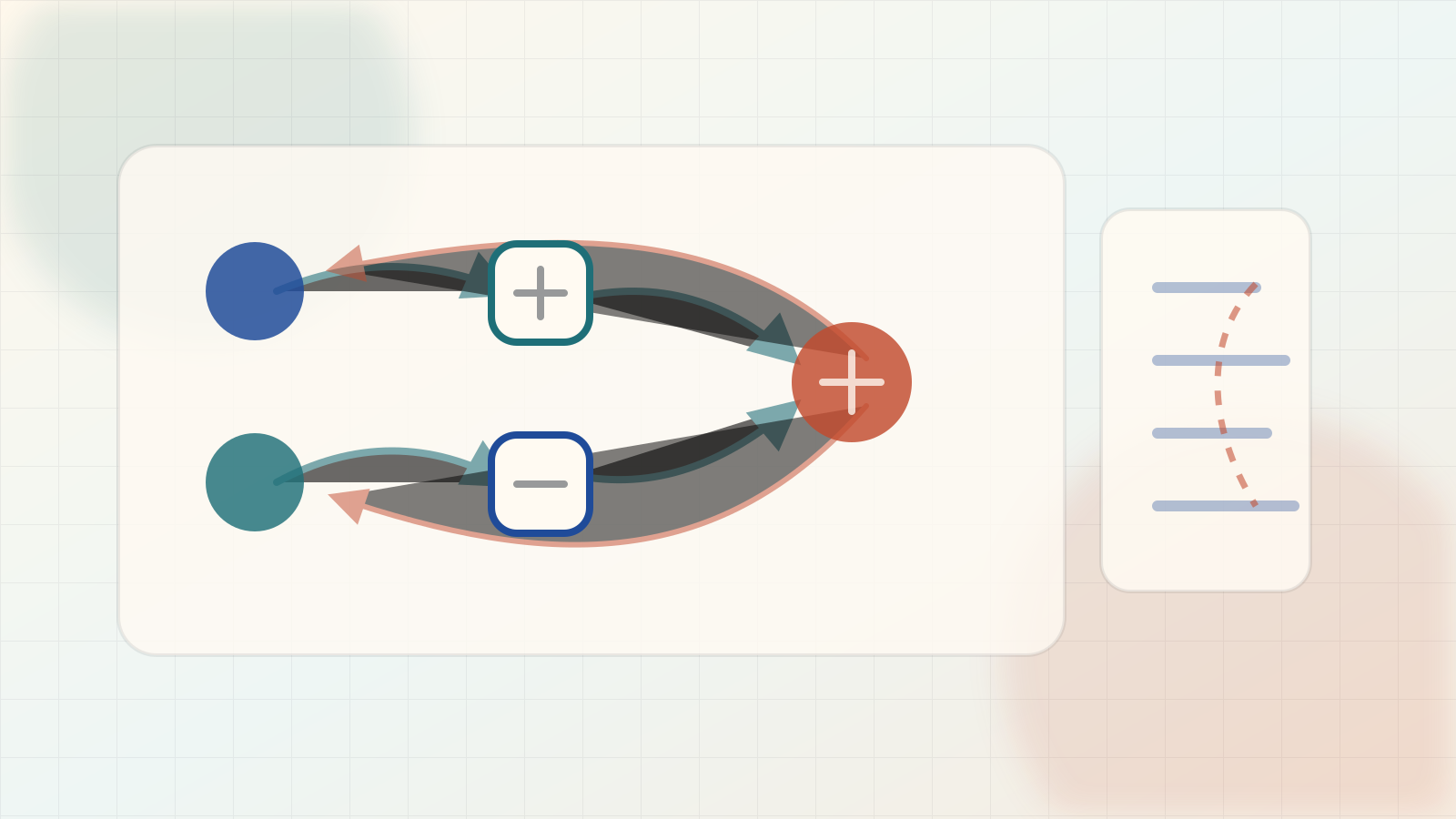
A computation graph breaks a calculation into nodes so values flow forward and sensitivities flow backward.

published · difficulty 2/5 · 13 min read

Intuition

Build the mental picture first so the rest of the page has something to attach to.

PredictName the object in plain language, then predict what should change.Leave with one reusable mental picture before notation appears.

Suppose one intermediate value gets used twice. If $a=xy$ , $b=\sin(a)$ , and $c=a+b$ , then $a$ affects $c$ directly and also through $b$ . How should the derivative remember both uses without differentiating one huge expanded formula by hand?

A computation graph makes that bookkeeping visible.

Instead of treating a function as one large expression, we split it into small operations: multiply here, apply a nonlinearity, add there, reuse an intermediate value. Each operation becomes a node, and each dependency becomes an edge.

A computation graph is not just an expression tree. The expanded expression $xy+\sin(xy)$ repeats $xy$ . The graph stores $a=xy$ once and records that two later operations depend on that same value.

This matters because the graph gives backpropagation a route. Values move forward through the graph to produce an output or loss. Derivatives move backward through the same graph, using local slopes on each edge. The chain rule stops feeling like one giant symbolic derivative and becomes bookkeeping over small local changes.

Section prompt

Copy-only prompts — each action copies a page-grounded prompt to your clipboard. Nothing is sent by this site.

Math

Translate the story into symbols, assumptions, and a derivation you can inspect.

InspectTrack the same object through the notation and check each symbol.Leave with the invariant the equations preserve.

Equation 1Inspect equation objecta = xy,\qquad b = \sin(a),\qquad c = a + b.Equation 2Inspect equation object\bar v = (\partial c)/(\partial v).Equation 3Inspect equation object\bar a \mathrel{+}= \bar c(\partial c)/(\partial a)\Big|_{direct} = 1,\qquad \bar b \mathrel{...

In this first example, every node is scalar. Let $x,y\in\mathbb R$ , and draw edges from inputs to the values that depend on them. The graph for one forward pass is a directed acyclic graph: later nodes depend on earlier nodes, not the other way around.

Consider the scalar computation

a = xy,\qquad b = \sin(a),\qquad c = a + b.

The graph has inputs $x,y$ , intermediate nodes $a,b$ , and output $c$ . The forward pass stores each node value. The important detail is reuse: $a$ is stored once, but two later uses depend on it. The backward pass asks how a small change in each node would affect the output.

For any node $v$ , write

\bar v = \frac{\partial c}{\partial v}.

The output seed is $\bar c=1$ . The final add node $c=a+b$ sends one unit of sensitivity to both inputs:

\bar a \mathrel{+}= \bar c\frac{\partial c}{\partial a}\Big|_{\text{direct}} = 1,\qquad \bar b \mathrel{+}= \bar c\frac{\partial c}{\partial b} = 1.

The sine branch also sends a local contribution into the same stored node $a$ . The important invariant is local: a node's cotangent is the sum of contributions from each immediate downstream use. The demo hides the sine-branch contribution until you predict whether it will lower, preserve, or raise the direct baseline.

The backward pass does not expand every symbolic path; each downstream node has already summarized everything beyond it.

For vector or tensor nodes, the same idea uses Jacobians or local vector-Jacobian product rules. With column-vector cotangents, if $v_j=f(v_i)$ and $J_{ji}=\partial v_j/\partial v_i$ , the reverse update is

\bar v_i \mathrel{+}= J_{ji}^{\mathsf T}\bar v_j.

Reverse-mode autodiff is the automated version of this bookkeeping: save forward values, then run local backward rules in reverse topological order.

Section prompt

Copy-only prompts — each action copies a page-grounded prompt to your clipboard. Nothing is sent by this site.

Code

Keep the implementation aligned with the notation so the algorithm is legible.

TraceMatch variables to symbols before reading the implementation.Leave with a runnable witness for the math.

Code witness 1import math x, y = 2.0, 3.0 # Forward pass: store intermediate node values. a = x * y b = mat...python

import math

x, y = 2.0, 3.0

# Forward pass: store intermediate node values.
a = x * y
b = math.sin(a)
c = a + b

# Reverse pass bookkeeping: every downstream use appends one local contribution.
bar_c = 1.0
bar_a = 0.0
bar_b = 0.0
bar_x = 0.0
bar_y = 0.0

# c = a + b sends one unit to both inputs.
bar_a += bar_c * 1.0
bar_b += bar_c * 1.0

# b = sin(a) sends another contribution into reused node a.
bar_a += bar_b * math.cos(a)

# a = x * y sends the accumulated sensitivity to x and y.
bar_x += bar_a * y
bar_y += bar_a * x

print("c:", round(c, 4))
print("stored a once:", a)
print("downstream uses of a:", ["direct add edge", "sine edge"])
print("bar_a:", round(bar_a, 4))
print("dc/dx:", round(bar_x, 4))
print("dc/dy:", round(bar_y, 4))

The code is deliberately manual. The += updates are the graph mechanism: a reused node collects every downstream local contribution before sending its accumulated sensitivity to its own inputs.

Section prompt

Copy-only prompts — each action copies a page-grounded prompt to your clipboard. Nothing is sent by this site.

Interactive Demo

Use direct manipulation to connect the explanation to a moving system.

ManipulateChange one control and predict the visible response before reveal.Leave with the observed invariant or a repaired model.

Live Concept Demo

Explore Computation Graphs

The stage is code-native and interactive. Use it to test the explanation against the mechanism.

difficulty 2/5undergraduatecode-aligned

Demo inquiry checkpoint

Manipulate one control and predict the visible change.

01Choose lensTrace a quantity

02ObserveDemo state pending

03GroundName the equation, invariant, or control that explains it.

04CarryNext: Reverse-Mode Automatic Differentiation

Choose what to inspect in Computation Graphs. This shared fallback is an observation guide, not evidence of learning.

Loading interactive demo...

Use the sliders to change $x$ and $y$ . In Forward mode, watch the stored value $a=xy$ feed both $b=\sin(a)$ and the final add node $c=a+b$ .

Before switching into the backward numbers, predict whether the hidden accumulated sensitivity at the reused node $a$ should land lower than, nearly equal to, or higher than the direct contribution from $c=a+b$ .

Use Case A and Case B as neutral graph states. Commit first, then reveal how the downstream paths combine before $a$ sends sensitivity back to $x$ and $y$ .

Section prompt

Copy-only prompts — each action copies a page-grounded prompt to your clipboard. Nothing is sent by this site.

Object

4/4 sections ready

Concept: Computation Graphs

What is the smallest example that makes Computation Graphs click without losing the math?

BeforeChain RuleNow4/4 sections readyTryManipulate one control and predict the visible change.NextReverse-Mode Automatic Differentiation

Object contextCalculus

StateCalculus

1 source attachedChecking local snapshot

concept:calculus/computation-graphs

Math3 equation objectsa = xy,\qquad b = \sin(a),\qquad c = a + b.CodeComputation Graphs code witness 1print("downstream uses of a:", ["direct add edge", "sine edge"])DemoComputation Graphs predictionManipulate one control and predict the visible change.

ConceptLearner lens

Computation Graphs

What is the smallest example that makes Computation Graphs click without losing the math?

Mode questionCan I say the mechanism back in one sentence before I reveal anything?

Start with the prediction checkpoint, then compare the reveal to the mental model.

Take this move

Study modes

Keep the object fixed; change the lens.

01PredictCommit before reveal.02ExplainName the invariant.03Ground1 source link nearby.04ExperimentChange one knob.05CarrySave the next question.

Route back through the notebook

Carry the same object through intuition, math, code, and demo.

4/4 sections ready

Carry inChain Rule

Bring the mental model from Chain Rule; this page will reuse it instead of restarting from zero.

Work hereComputation Graphs

A computation graph breaks a calculation into nodes so values flow forward and sensitivities flow backward.

Carry outReverse-Mode Automatic Differentiation

The next edge should feel earned: use the demo prediction here before following Reverse-Mode Automatic Differentiation.

After The First Pass

Turn the concept into an inspected object.

The lower panels are one second act: keep the object fixed, inspect it visually, check source boundaries, practice transfer, then attach the research question.

ConceptComputation GraphsCalculus

01MechanismInspect motionSee how the idea changes form before adding more explanation.02VisualChoose a cueBind one visible mark to one mathematical role.03SourcesCheck boundary1 source link attached to the object.04ClaimAudit evidenceTreat the page claim as something to verify.05PracticeAttempt transferWrite before feedback so the model has something to repair.06RoomAsk groundedAttach the question to the same exact object.

Mechanism Storyboard

See the idea move before the page explains it

A computation graph breaks a calculation into nodes so values flow forward and sensitivities flow backward.

Demo notes open01 / Intuition

Editorial autodiff illustration of computation graph nodes with forward value flow and backward sensitivity arrows.

Prediction lens

Start with the picture, metaphor, or geometric mechanism.

Commit first

Before reading further, choose the kind of change Computation Graphs should make visible.

Visual Inquiry

Make the image answer a mathematical question

A computation graph breaks a calculation into nodes so values flow forward and sensitivities flow backward.

4/4 stages readyDemo notes connected

Visual cueWhich visible object should carry the first intuition?

Inspection depth2/4

Prediction

Which visible object should carry the first intuition?

Commit first

Pick the cue that should make Computation Graphs easier to reason about before the page gives the answer.

Source Grounding

Canonical references for the mechanism on this page.

Object - ConceptComputation GraphsQuestion

What is the smallest example that makes Computation Graphs click without losing the math?

concept:calculus/computation-graphs

Boundary

sources: baydin-2018-ad-survey

Check

Open the closest source note before trusting the local explanation.

Evidence

1 selected-object source shown first; 1 reference total.

Next move

Audit the claim boundary, then ask from the same selected object.

selected object source · paper · 2018Automatic differentiation in machine learning: a surveyBaydin et al.

Located CF editorial boundary

Grounds computation graphs as the program structure used by automatic differentiation systems.

Used here as

Baydin et al. describe AD over evaluation traces of elementary operations, computational graphs for dependency relations, and reverse mode as a forward pass that populates intermediate va...

Caveat

Covers differentiable primitives in one executed DAG/program trace and local scalar/vector-VJP teaching model, not symbolic simplification, mutation/aliasing, checkpointing policy, nonsmo...

Open source

Claim Review

A computation graph breaks a calculation into nodes so values flow forward and sensitivities flow backward.

Object - ConceptComputation GraphsQuestion

What is the smallest example that makes Computation Graphs click without losing the math?

concept:calculus/computation-graphs

Boundary

sources: baydin-2018-ad-survey

Check

Treat every claim as provisional until source support and a local witness agree.

Evidence

1 structured claim check on this concept.

Next move

Run the prediction or practice transfer before asking for a grounded review.

1 CF editorial source-scope review recorded

Publisher-side editorial review is not independent replication. Claims without it still need exact source-support review. 1 reference and 3 local witnesses are available for inspection.

For one executed differentiable program, a computation graph uses elementary-operation nodes and dependency edges, stores each reused intermediate node value once in the forward pass, and makes reverse-mode/backprop local: downstream sensitivities from every use accumulate at a node before being sent to its inputs.

Registered CF editorial boundary

Automatic differentiation in machine learning: a surveyGrounds computation graphs as the program structure used by automatic differentiation systems.

Used here as

Baydin et al. describe AD over evaluation traces of elementary operations, computational graphs for dependency relations, and reverse mode as a forward pass that populates intermediate variables/records grap...

Local witness

source-span-baydin-2018-ad-survey math-object-1 math-object-2 code-witness-1 interactive-demo

Equation 1

a = xy,\qquad b = \sin(a),\qquad c = a + b.

Equation 2

\bar v = \frac{\partial c}{\partial v}.

Caveat

Covers differentiable primitives in one executed DAG/program trace and local scalar/vector-VJP teaching model, not symbolic simplification, mutation/aliasing, checkpointing policy, nonsmooth primitives, or e...

Review stateCF editorial source-scope reviewClaim metadata: source checkedPublisher-side editorial review only; not independent replication. Check caveats and exact source scope.

Checked Baydin et al. for one executed AD trace: programs become elementary-operation traces and graphs of intermediate-variable dependencies; reverse mode runs code forward, populates intermediates, records dependencies, then propagates adjoints backward; a reused variable's adjoint sums downstream contributions before input derivatives are obtained. Local math/code/demo instantiate a=xy,b=sin(a),c=a+b with one stored a, direct + sine-path cotangent accumulation, and propagation to x,y.

Reviewer: codex+oracle; reviewed 2026-05-07

Practice notebook

Use the idea, then test it somewhere new

A computation graph breaks a calculation into nodes so values flow forward and sensitivities flow backward.

AttemptNo learning claim inferred

Object - ConceptComputation GraphsQuestion

What is the smallest example that makes Computation Graphs click without losing the math?

concept:calculus/computation-graphs

Boundary

sources: baydin-2018-ad-survey

Check

Use one state from Computation Graphs to explain what changes, why it changes, and which assumption the explanation needs.

Evidence

No learner move yet; no learning state is inferred.

Next move

Write first, use only the help you need, then try a new case without it.

Explain

Use one state from Computation Graphs to explain what changes, why it changes, and which assumption the explanation needs.

Hint 1

Reveal when your model needs a nudge.

Hint 2

Reveal when your model needs a nudge.

Hint 3

Reveal when your model needs a nudge.

Your answer canvas

Attempt context

Learner move

Write an attempt before asking the companion.

Assistance used

0 of 3 progressive hints opened.

Evidence boundary

This draft and any AI response do not establish mastery; a later unassisted case can.

Misconception check

Grounded object roomClose

Selected object routeAsk from this object; carry one invariant back.sources: baydin-2018-ad-survey

ObjectConceptComputation Graphs
PredictBefore revealComputation Graphs prediction
WitnessCompare codeComputation Graphs code witness 1
RoomAsk groundedChecking local snapshot

ConceptComputation GraphsCalculus

Code witness comparisonComputation Graphs code witness 1print("downstream uses of a:", ["direct add edge", "sine edge"])Prediction before revealComputation Graphs predictionManipulate one control and predict the visible change.

Grounded room questionWhat is the smallest example that makes Computation Graphs click without losing the math?Checking local snapshot

Research Room

Attach the question to an exact object

Pick the concept, equation, source, code witness, claim, misconception, or demo state before asking for help. The handoff stays grounded to that object.

Next local actionNo local draft saved yet

Open the draft below to save one note and next action in this browser.

conceptCalculus

Computation Graphs

Anchored question

What is the smallest example that makes Computation Graphs click without losing the math?

Source boundaryInspect source ids: baydin-2018-ad-surveyStable content-object key attached

Role lenses for this object

These are fixed, deterministic perspectives derived from the selected object. They do not represent people, community contributions, or independent review.

Learner evidence requestAsk what would make "Computation Graphs" feel predictable rather than familiar.

Assumption

Source ids baydin-2018-ad-survey must support the exact object, not just the surrounding topic.

Source-checking summary

Treat this as a mechanism object: connect the definition to one equation, code witness, or demo before broadening the discussion.

Proposed experiment

Ask the learner to perturb one representation, then check whether the same invariant survives in math, code, and demo.

Next action

The learner can state the mechanism in their own words

Evidence4 checks

PredictionChecking carried observation

ActionReady for one action

AILearner handoff ready

Open source object

01PredictionChecking browser-local route memory

02EvidenceChecking for a carried observation

03BoundaryInspect source ids: baydin-2018-ad-survey

04Next moveSave one next action

Local action draftNo local draft saved yetExpand only when ready to capture one local next action

Local action draft

This draft stays locally in this browser for concept:calculus/computation-graphs.

Draft noteNext action

No local draft saved.

Evidence to inspect

Source ids to inspect: baydin-2018-ad-survey
Definition, prerequisite, and contrast concept links
The equation or code witness that makes the concept operational
One demo state that shows the invariant instead of a slogan

What would resolve this

The learner can state the mechanism in their own words
The learner can name the prerequisite that would repair confusion
The learner can predict how the mechanism changes under one perturbation

Object-attached AI handoff

I am working in Continuous Function's research reading room. Object: concept - Computation Graphs Object key: concept:calculus/computation-graphs Context: Calculus Anchor id: concept/concept-notebook/calculus/computation-graphs Open question: What is the smallest example that makes Computation Graphs click without losing the math? Evidence to inspect: - Source ids to inspect: baydin-2018-ad-survey - Definition, prerequisite, and contrast concept links - The equation or code witness that makes the concept operational - One demo state that shows the invariant instead of a slogan Deterministic role lenses for this object: - Boundary: fixed perspectives, not people, community contributions, or independent review - Source-checking summary: Treat this as a mechanism object: connect the definition to one equation, code witness, or demo before broadening the discussion. - Proposed experiment: Ask the learner to perturb one representation, then check whether the same invariant survives in math, code, and demo. - Teach/transfer move: Turn the mechanism into one sentence that predicts a neighboring concept. - Assumptions: - Source ids baydin-2018-ad-survey must support the exact object, not just the surrounding topic. - The stable content-object key lets local drafts, prompts, and route memory attach without changing the source page. - The concept explanation is local atlas prose until checked against its math, code, and source support. - Prerequisite gaps should become a repair route, not a reason to leave the object vague. - Role-lens requests: - Learner: ask for "Ask what would make "Computation Graphs" feel predictable rather than familiar." | assumption: Source ids baydin-2018-ad-survey must support the exact object, not just the surrounding topic. | next action: The learner can state the mechanism in their own words - Researcher: ask for "Source ids to inspect: baydin-2018-ad-survey" | assumption: The stable content-object key lets local drafts, prompts, and route memory attach without changing the source page. | next action: The learner can name the prerequisite that would repair confusion - Experimenter: ask for "Choose one variable or condition to perturb before asking for an explanation." | assumption: The concept explanation is local atlas prose until checked against its math, code, and source support. | next action: The learner can predict how the mechanism changes under one perturbation - Professor: ask for "Find the smallest transferable rule a learner could reuse without the AI." | assumption: Prerequisite gaps should become a repair route, not a reason to leave the object vague. | next action: Teach or transfer: Turn the mechanism into one sentence that predicts a neighboring concept. What would resolve this: - The learner can state the mechanism in their own words - The learner can name the prerequisite that would repair confusion - The learner can predict how the mechanism changes under one perturbation Answer as a careful research tutor: stay source-grounded, separate verified evidence from assumptions, name the relevant math objects, and end with one next action. Current deterministic role lens for this object: - Role lens: Learner - Evidence request: Ask what would make "Computation Graphs" feel predictable rather than familiar. - Assumption to keep visible: Source ids baydin-2018-ad-survey must support the exact object, not just the surrounding topic. - Proposed experiment: Ask the learner to perturb one representation, then check whether the same invariant survives in math, code, and demo. - Next action: The learner can state the mechanism in their own words

concept/concept-notebook/calculus/computation-graphs
concept:calculus/computation-graphs

Learning Map

Before / Now / Try / Next

BeforeChain Rule

NowIntuition → Math → Code → Demo

TryManipulate one control and predict the visible change.

NextReverse-Mode Automatic Differentiation

Learnerpicture first Researchersource check Experimentertest the demo Professorname invariant

01Predict 02Ground 03Code 04Carry

01Intuitionready
02Mathready
03Codeready
04Interactive Demoready

Object Companion

Ask beside the selected object

A computation graph breaks a calculation into nodes so values flow forward and sensitivities flow backward.

Your question

GoalComfortStyleStuck on

Context prompt

You are my AI learning companion for Continuous Function. Current context: Calculus concept. Learning surface: Computation Graphs. What this page says: A computation graph breaks a calculation into nodes so values flow forward and sensitivities flow backward. Current section: Intuition, math, code, and interactive demo. Suggested next step: Manipulate one control and predict the visible change.. Learner goal: Understand the idea. Learner comfort level: New to this. Preferred explanation style: Visual first. Task: Explain the central idea in plain language, then restate it with the exact math objects from the page. Answer in a way that helps me learn: ask one clarifying question only if needed, use intuition before notation, and end with one thing I should try on the page.

Copy-only tool: this panel composes a prompt for an AI tool you already use. Nothing you enter here is sent from this page.

Domain

Calculus

calculusautodiffbackpropagation

Prerequisites

Chain Rule

Leads To

Reverse-Mode Automatic Differentiation

Backpropagation

Within this domain