Bring the mental model from Computation Graphs; this page will reuse it instead of restarting from zero.
Calculus
Reverse-Mode Automatic Differentiation
Reverse-mode autodiff computes gradients by sending cotangents backward through a computation graph.
Concept Structure
Reverse-Mode Automatic Differentiation
01Intuition
Start with the picture, metaphor, or geometric mechanism.
02Math
Make the objects explicit and connect them with notation.
03Code
Mirror the equations with runnable implementation details.
04Interactive Demo
Manipulate the mechanism and watch the idea respond.
1prerequisites
1next concepts
2related links
Learning map
Reverse-Mode Automatic DifferentiationBeforeComputation GraphsNow4/4 sections readyTryManipulate one control and predict the visible change.NextBackpropagation
Conceptual Bridge
What should feel connected as you move through this page.
Reverse-mode autodiff computes gradients by sending cotangents backward through a computation graph.
The next edge should feel earned: use the demo prediction here before following Backpropagation.
Test the linkManipulate one control and predict the visible change.Then continue to Backpropagation
01IntuitionStart with the picture, metaphor, or geometric mechanism.02MathMake the objects explicit and connect them with notation.03CodeMirror the equations with runnable implementation details.04Interactive DemoManipulate the mechanism and watch the idea respond.
01
01
Intuition
Build the mental picture first so the rest of the page has something to attach to.
Section prompt
Suppose one scalar loss depends on millions of parameters. Do you need to run one derivative computation for each parameter to know how to change them all?
Reverse-mode automatic differentiation is the bookkeeping trick that makes the answer no.
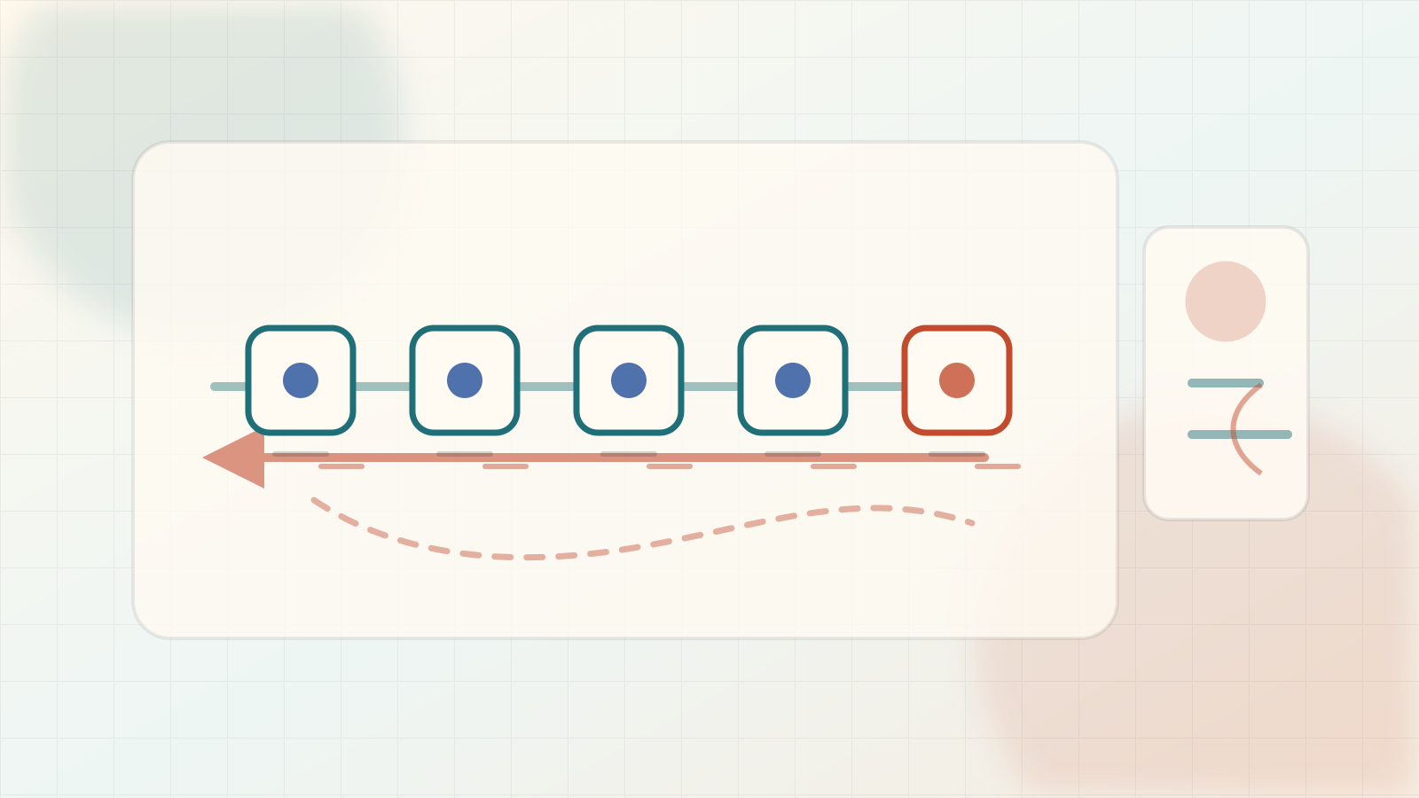
The previous idea, computation graphs, makes dependencies visible. Reverse-mode AD adds an execution rule: during the forward pass, record the primitive operations and the intermediate values they will need later. During the reverse pass, start from the final question, "how much does the loss change if this output changes?", and walk backward through the recorded operations. Each local backward rule converts an output sensitivity into input sensitivities.
The key advantage is shape. If one scalar loss depends on many parameters, reverse mode can compute all parameter gradients in one backward sweep through the graph. Forward mode would ask, one input direction at a time, how the output changes.
The useful mental model is a tape plus a register file. The tape remembers what primitive operations ran. The registers store cotangents such as and . The model breaks if you imagine symbolic simplification: reverse mode does not expand the formula by hand; it accumulates local contributions on the graph that actually ran.
02
02
Math
Translate the story into symbols, assumptions, and a derivation you can inspect.
Section prompt
Equation 1\bar v_i = \frac{\partial L}{\partial v_i}.Equation 2\bar L = \frac{\partial L}{\partial L} = 1.
Let a differentiable computation graph produce a scalar output from intermediate variables . Reverse mode stores, for each node, an adjoint or cotangent
Before the reverse sweep, initialize every non-output cotangent register to zero. Then seed the scalar output with
For scalar nodes and a local operation , the chain rule sends sensitivity backward. When the operation producing is processed, already contains all downstream contributions:
For an operation with multiple inputs, such as , each input receives its own local derivative:
The plus-equals matters. If a value is reused by several later nodes, all downstream paths contribute to its total sensitivity. Reverse mode is therefore not symbolic simplification; it is graph-local accumulation of vector-Jacobian products.
For vector nodes, choose column-vector cotangents. If , , , , and
then the reverse update is
This is the direction contrast:
For a scalar loss , one forward evaluation records the needed values, and one reverse sweep gives the full gradient
assuming primitive backward rules are available. The cost is memory for saved forward values on a tape, or extra compute if some values are recomputed. An autodiff engine automates this bookkeeping by recording primitive operations during the forward pass and executing their local backward rules in reverse topological order.
These equations assume the recorded primitives are differentiable at the saved forward values. For nonsmooth primitives, an implementation must choose a convention, use a subgradient, or report that the derivative is undefined. If the program has control flow, reverse mode differentiates the branch that actually ran.
03
03
Code
Keep the implementation aligned with the notation so the algorithm is legible.
Section prompt
import math

x, y = 2.0, 3.0

# Forward graph:
# a = x * y
# b = sin(a)
# L = a + b
a = x * y
b = math.sin(a)
L = a + b

# Reverse-mode table: each bar_* stores dL/d(node).
# Start with empty cotangent registers, then seed the output.
bar_L = 0.0
bar_a = 0.0
bar_b = 0.0
bar_x = 0.0
bar_y = 0.0

bar_L = 1.0

# Read the tape backward.
# L = a + b sends one unit of sensitivity to both inputs.
bar_a += bar_L * 1.0
bar_b += bar_L * 1.0

# b = sin(a) contributes another path back into a.
bar_a += bar_b * math.cos(a)

# a = x * y sends sensitivity to both inputs.
bar_x += bar_a * y
bar_y += bar_a * x

print("L:", round(L, 4))
print("dL/dx:", round(bar_x, 4))
print("dL/dy:", round(bar_y, 4))
The code initializes every cotangent register and then uses += for local contributions. The reused node receives two contributions: directly through , and indirectly through . With and , the output is approximately , , and .
04
04
Interactive Demo
Use direct manipulation to connect the explanation to a moving system.
Section prompt
Use the sliders to change and , then compare the three phases.
Forward tape mode records the primitive operations and the saved values that local backward rules will need. Reverse sweep mode reads the same tape backward, starts from , and fills the cotangent registers. Cost shape mode highlights the main reason reverse mode matters for deep learning: when many inputs feed one scalar loss, one reverse sweep gives the whole gradient vector.
Try the second preset after making a prediction. It changes the product regime so the same tape can expose a different cotangent-accumulation pattern.
Live Concept Demo
Explore Reverse-Mode Automatic Differentiation
The stage is code-native and interactive. Use it to test the explanation against the mechanism.
difficulty 3/5undergraduatecode-aligned
Demo Prediction Checkpoint
Manipulate one control and predict the visible change.
Commit to what Reverse-Mode Automatic Differentiation should make visible before reading the result.
After The First Pass
Turn the concept into an inspected object.
Once the invariant is visible in the intuition, math, code, and demo, use these panels to inspect the mechanism visually, check source support, practice the idea, and attach a grounded research question.
Mechanism Storyboard
See the idea move before the page explains it
Reverse-mode autodiff computes gradients by sending cotangents backward through a computation graph.
Prediction open01 / Intuition
Prediction lens
Start with the picture, metaphor, or geometric mechanism.
Commit first
Before reading further, choose the kind of change Reverse-Mode Automatic Differentiation should make visible.
Visual Inquiry
Make the image answer a mathematical question
Reverse-mode autodiff computes gradients by sending cotangents backward through a computation graph.
4/4 stages readyLive demo connected
Visual cueWhich visible object should carry the first intuition?
Prediction
Which visible object should carry the first intuition?
Commit first
Pick the cue that should make Reverse-Mode Automatic Differentiation easier to reason about before the page gives the answer.
Source Grounding
Canonical references for the mechanism on this page.
Grounds reverse mode as the efficient way to compute gradients of scalar losses with many parameters.
Open sourceClaim Review
Reverse-mode autodiff computes gradients by sending cotangents backward through a computation graph.
Claims without a substantive review badge still need exact source-support review.
baydin-2018-ad-survey
Use equation, code, and demo objects to check whether the source support is operational.
Baydin et al. describe reverse mode as running code forward to populate intermediate variables and record graph dependencies, then propagating adjoints backward. Their example shows incremental adjoint accumulation and output adjoint 1; they state that for f:R^n->R one reverse-mode application computes the full gradient, matching scalar-valued ML objectives with many parameters.
Sources: Automatic differentiation in machine learning: a surveyChecks reverse-mode bookkeeping for one executed differentiable computation: forward tape/saved values, then reverse cotangent sweep with primitive backward rules. Not checkpointing, recomputation, nonsmooth primitives, control flow, framework edge cases, or higher derivatives.A bounded review summary is present; still check caveats and exact source scope.Checked Baydin et al. 3.2: reverse mode runs code forward to populate intermediates and record dependencies, then propagates adjoints backward. The example starts from output adjoint 1, accumulates reused-variable cotangents from downstream paths, and gets both input derivatives in one reverse pass. Baydin says for f:R^n->R one reverse application computes the full gradient. Local witnesses match tape values, bar L=1, += pullbacks, VJP/J^T notation, and scalar-loss shape.
Reviewer: codex+oracle; reviewed 2026-05-07Practice Loop
Try the idea before it explains itself
Reverse-mode autodiff computes gradients by sending cotangents backward through a computation graph.
Readiness0/3 checks ready
Predict
Before touching the demo, predict one visible change that should happen in Reverse-Mode Automatic Differentiation.
Hint 1
Reveal when your model needs a nudge.
Hint 2
Reveal when your model needs a nudge.
Hint 3
Reveal when your model needs a nudge.
Local checks
Claim
A concrete answer is on the canvas.
Mechanism
The answer names why the claim should hold.
Bridge
It touches the page context or a neighboring idea.
Object research drawerClose
ConceptReverse-Mode Automatic DifferentiationCalculus
Code witness comparisonReverse-Mode Automatic Differentiation code witness 1x, y = 2.0, 3.0Prediction before revealReverse-Mode Automatic Differentiation interactive demoManipulate one control and predict the visible change.
Grounded room questionWhat is the smallest example that makes Reverse-Mode Automatic Differentiation click without losing the math?Local snapshot ready
Research Room
Attach the question to an exact object
Pick the concept, equation, source, code witness, claim, misconception, or demo state before asking for help. The handoff stays grounded to that object.Open the draft below to save one note and next action in this browser.
Reverse-Mode Automatic Differentiation
Anchored question
What is the smallest example that makes Reverse-Mode Automatic Differentiation click without losing the math?
Local action draftNo local draft saved yetExpand only when ready to capture one local next action
Local action draft
This draft stays locally in this browser for concept:calculus/reverse-mode-autodiff.
No local draft saved.
- Source ids to inspect: baydin-2018-ad-survey
- Definition, prerequisite, and contrast concept links
- The equation or code witness that makes the concept operational
- One demo state that shows the invariant instead of a slogan
- The learner can state the mechanism in their own words
- The learner can name the prerequisite that would repair confusion
- The learner can predict how the mechanism changes under one perturbation
Grounded AI handoff
I am working in Continuous Function's research reading room. Object: concept - Reverse-Mode Automatic Differentiation Object key: concept:calculus/reverse-mode-autodiff Context: Calculus Anchor id: concept/concept-notebook/calculus/reverse-mode-autodiff Open question: What is the smallest example that makes Reverse-Mode Automatic Differentiation click without losing the math? Evidence to inspect: - Source ids to inspect: baydin-2018-ad-survey - Definition, prerequisite, and contrast concept links - The equation or code witness that makes the concept operational - One demo state that shows the invariant instead of a slogan What would resolve this: - The learner can state the mechanism in their own words - The learner can name the prerequisite that would repair confusion - The learner can predict how the mechanism changes under one perturbation Answer as a careful research tutor: stay source-grounded, separate verified evidence from assumptions, name the relevant math objects, and end with one next action.
concept/concept-notebook/calculus/reverse-mode-autodiff
concept:calculus/reverse-mode-autodiff