Bring the mental model from Derivatives; this page will reuse it instead of restarting from zero.
Optimization
Gradient Descent
Gradient descent turns local slope information into an iterative update rule for reducing a loss.
Concept Structure
Gradient Descent
01Intuition
Start with the picture, metaphor, or geometric mechanism.
02Math
Make the objects explicit and connect them with notation.
03Code
Mirror the equations with runnable implementation details.
04Interactive Demo
Manipulate the mechanism and watch the idea respond.
1prerequisites
3next concepts
3related links
Learning map
Gradient DescentBeforeDerivativesNow4/4 sections readyTryManipulate one control and predict the visible change.NextSGD & Momentum: The Workhorses of Optimization
Conceptual Bridge
What should feel connected as you move through this page.
Gradient descent turns local slope information into an iterative update rule for reducing a loss.
The next edge should feel earned: use the demo prediction here before following SGD & Momentum: The Workhorses of Optimization.
Test the linkManipulate one control and predict the visible change.Then continue to SGD & Momentum: The Workhorses of Optimization
01IntuitionStart with the picture, metaphor, or geometric mechanism.02MathMake the objects explicit and connect them with notation.03CodeMirror the equations with runnable implementation details.04Interactive DemoManipulate the mechanism and watch the idea respond.
01
01
Intuition
Build the mental picture first so the rest of the page has something to attach to.
Section prompt
A model can receive one scalar complaint, the loss is high, while having thousands or millions of parameters. Which way should those parameters move?
Gradient descent is the basic answer behind most neural-network training: measure which way the loss rises, then step the other way.
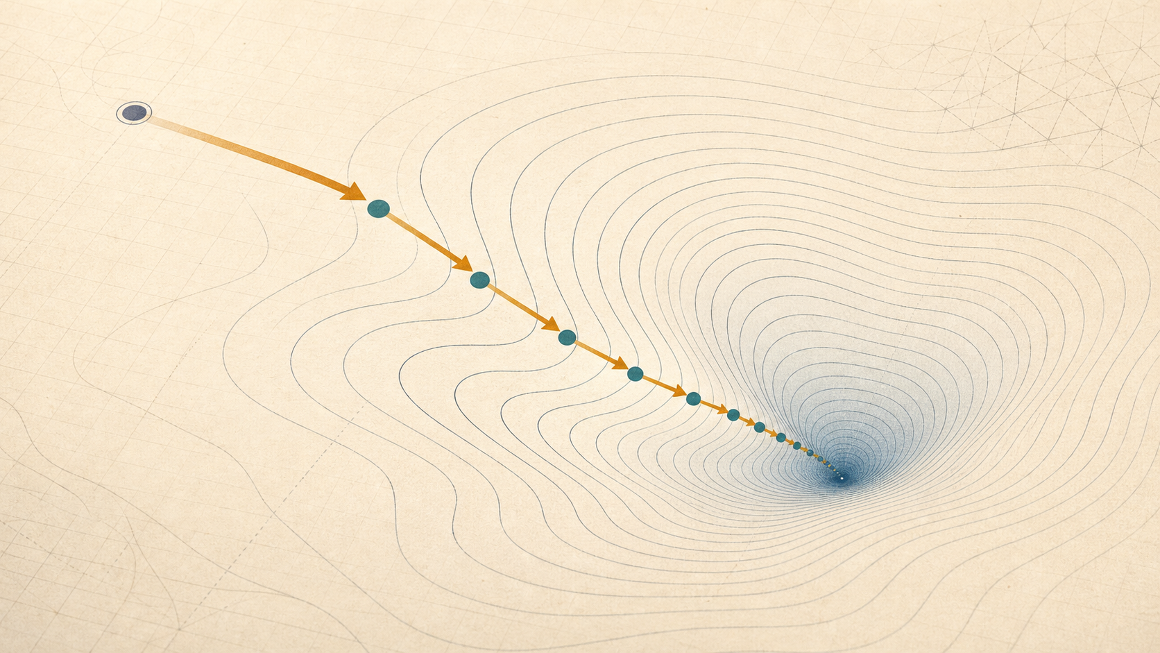
Imagine standing on a landscape in fog. You cannot see the whole terrain, but you can feel the local slope under your feet. The gradient points in the steepest uphill direction. If your goal is to lower the loss, you walk against that direction.
The method is deliberately local. It does not know whether a better valley exists far away, and it can move too slowly or overshoot if the step size is wrong. But it gives a reusable training loop: compute a loss, differentiate it, update parameters, repeat.
This page assumes the gradient is already available. Backpropagation explains how computation graphs and reverse-mode autodiff produce that gradient for neural networks; gradient descent explains how an optimizer consumes it.
02
02
Math
Translate the story into symbols, assumptions, and a derivation you can inspect.
Section prompt
Equation 1\nabla_\theta L(\theta_t)Equation 2\theta_{t+1} = \theta_t - \eta \nabla_\theta L(\theta_t),
Let be a loss function and let be the current parameter vector. Under the standard Euclidean inner product, the gradient
points in the direction of steepest local increase. Gradient descent uses the update
where is the learning rate.
If is differentiable near and , the first-order Taylor approximation says
That is the local reason stepping against the gradient should reduce the loss. The learning rate controls how much you trust this local approximation. If is too small, training makes slow progress. If is too large, the update can jump across a valley or even increase the loss. On a quadratic loss, this tradeoff is governed by curvature: steep directions demand smaller stable steps than flat directions.
At a stationary point, , so this first-order decrease argument disappears. In a nonconvex loss, such a point might be a minimum, a saddle, or a maximum.
For the quadratic used below,
with symmetric positive definite, the gradient is . In an eigen-direction of with curvature , the update becomes
Fixed-step descent is stable only when for every direction, so
This is the stability bound used by the code and the demo.
In deep learning, the exact gradient over the whole dataset is often too expensive. For a training set of examples, define the empirical risk
For a mini-batch , we instead compute
With uniform sampling, estimates . That turns gradient descent into stochastic gradient descent. The update is the same shape, but the direction is noisy:
03
03
Code
Keep the implementation aligned with the notation so the algorithm is legible.
Section prompt
import numpy as np

# Minimize L(theta) = 0.5 * theta^T A theta.
# The second coordinate has much higher curvature.
# Shapes: A is (2, 2), theta is (2,), grad(theta) is (2,).
A = np.diag([1.0, 20.0])
theta = np.array([5.0, 5.0])
lr = 0.08

def loss(theta):
    return 0.5 * theta @ A @ theta

def grad(theta):
    return A @ theta

for step in range(20):
    theta = theta - lr * grad(theta)
    if step in [0, 1, 2, 5, 19]:
        print(step + 1, "theta=", np.round(theta, 3), "loss=", round(loss(theta), 3))
For this quadratic, , so stable fixed-step descent needs . Try lr = 0.005, 0.08, and 0.12 to see slow movement, stable zig-zagging, and instability.
04
04
Interactive Demo
Use direct manipulation to connect the explanation to a moving system.
Section prompt
Use the learning-rate slider on the stretched quadratic bowl. The contours show the loss, the blue path shows repeated gradient-descent updates, and the brown arrow shows the first local step.
The presets start with the same high curvature as the code example, , so is stable while is not. The key comparison is the learning rate against the stability bound for this quadratic. A tiny learning rate crawls. A large but stable learning rate zig-zags across the high-curvature direction while still reducing loss. A learning rate above the bound eventually escapes instead of descending.
Change curvature while keeping the same learning rate. The gradient formula has not changed, but the safe step size has: steeper curvature makes the local slope become stale faster.
Live Concept Demo
Explore Gradient Descent
The stage is code-native and interactive. Use it to test the explanation against the mechanism.
difficulty 2/5undergraduatecode-aligned
Demo Prediction Checkpoint
Manipulate one control and predict the visible change.
Commit to what Gradient Descent should make visible before reading the result.
After The First Pass
Turn the concept into an inspected object.
Once the invariant is visible in the intuition, math, code, and demo, use these panels to inspect the mechanism visually, check source support, practice the idea, and attach a grounded research question.
Mechanism Storyboard
See the idea move before the page explains it
Gradient descent turns local slope information into an iterative update rule for reducing a loss.
Prediction open01 / Intuition
Prediction lens
Start with the picture, metaphor, or geometric mechanism.
Commit first
Before reading further, choose the kind of change Gradient Descent should make visible.
Visual Inquiry
Make the image answer a mathematical question
Gradient descent turns local slope information into an iterative update rule for reducing a loss.
4/4 stages readyLive demo connected
Visual cueWhich visible object should carry the first intuition?
Prediction
Which visible object should carry the first intuition?
Commit first
Pick the cue that should make Gradient Descent easier to reason about before the page gives the answer.
Source Grounding
Canonical references for the mechanism on this page.
Grounds descent methods, gradients, step sizes, and convex-optimization intuition.
Open sourceGrounds gradient-based learning as the optimization language used by neural networks.
Open sourceClaim Review
Gradient descent turns local slope information into an iterative update rule for reducing a loss.
Claims without a substantive review badge still need exact source-support review.
boyd-2004-convex-optimization, goodfellow-2016-deep-learning
Use equation, code, and demo objects to check whether the source support is operational.
Boyd and Vandenberghe ground descent methods, gradients, and step-size reasoning in convex optimization; Goodfellow et al. frame neural-network training as optimizing parameters of a cost function with gradient-based methods.
Sources: Convex Optimization, Deep LearningThis checks the local first-order update mechanism, not a guarantee of global convergence for nonconvex neural-network losses.A bounded review summary is present; still check caveats and exact source scope.Checked Goodfellow et al. chapters 4.3 and 8.3 plus Boyd/Vandenberghe chapter 9: Goodfellow gives directional derivative u^T grad f, says -grad is downhill, gives x' = x - eps grad f with eps as positive learning rate, and uses Taylor expansion to show curvature can make too-large steps move uphill. Boyd frames descent as direction plus step size and states Euclidean steepest descent coincides with gradient descent.
Reviewer: codex+oracle; reviewed 2026-05-06Practice Loop
Try the idea before it explains itself
Gradient descent turns local slope information into an iterative update rule for reducing a loss.
Readiness0/3 checks ready
Predict
Before touching the demo, predict one visible change that should happen in Gradient Descent.
Hint 1
Reveal when your model needs a nudge.
Hint 2
Reveal when your model needs a nudge.
Hint 3
Reveal when your model needs a nudge.
Local checks
Claim
A concrete answer is on the canvas.
Mechanism
The answer names why the claim should hold.
Bridge
It touches the page context or a neighboring idea.
Object research drawerClose
ConceptGradient DescentOptimization
Code witness comparisonGradient Descent code witness 1A = np.diag([1.0, 20.0])Prediction before revealGradient Descent interactive demoManipulate one control and predict the visible change.
Grounded room questionWhat is the smallest example that makes Gradient Descent click without losing the math?Local snapshot ready
Research Room
Attach the question to an exact object
Pick the concept, equation, source, code witness, claim, misconception, or demo state before asking for help. The handoff stays grounded to that object.Open the draft below to save one note and next action in this browser.
Gradient Descent
Anchored question
What is the smallest example that makes Gradient Descent click without losing the math?
Local action draftNo local draft saved yetExpand only when ready to capture one local next action
Local action draft
This draft stays locally in this browser for concept:optimization/gradient-descent.
No local draft saved.
- Source ids to inspect: boyd-2004-convex-optimization, goodfellow-2016-deep-learning
- Definition, prerequisite, and contrast concept links
- The equation or code witness that makes the concept operational
- One demo state that shows the invariant instead of a slogan
- The learner can state the mechanism in their own words
- The learner can name the prerequisite that would repair confusion
- The learner can predict how the mechanism changes under one perturbation
Grounded AI handoff
I am working in Continuous Function's research reading room. Object: concept - Gradient Descent Object key: concept:optimization/gradient-descent Context: Optimization Anchor id: concept/concept-notebook/optimization/gradient-descent Open question: What is the smallest example that makes Gradient Descent click without losing the math? Evidence to inspect: - Source ids to inspect: boyd-2004-convex-optimization, goodfellow-2016-deep-learning - Definition, prerequisite, and contrast concept links - The equation or code witness that makes the concept operational - One demo state that shows the invariant instead of a slogan What would resolve this: - The learner can state the mechanism in their own words - The learner can name the prerequisite that would repair confusion - The learner can predict how the mechanism changes under one perturbation Answer as a careful research tutor: stay source-grounded, separate verified evidence from assumptions, name the relevant math objects, and end with one next action.
concept/concept-notebook/optimization/gradient-descent
concept:optimization/gradient-descent