Bring the mental model from Distributions; this page will reuse it instead of restarting from zero.
Probability
Bayesian Inference
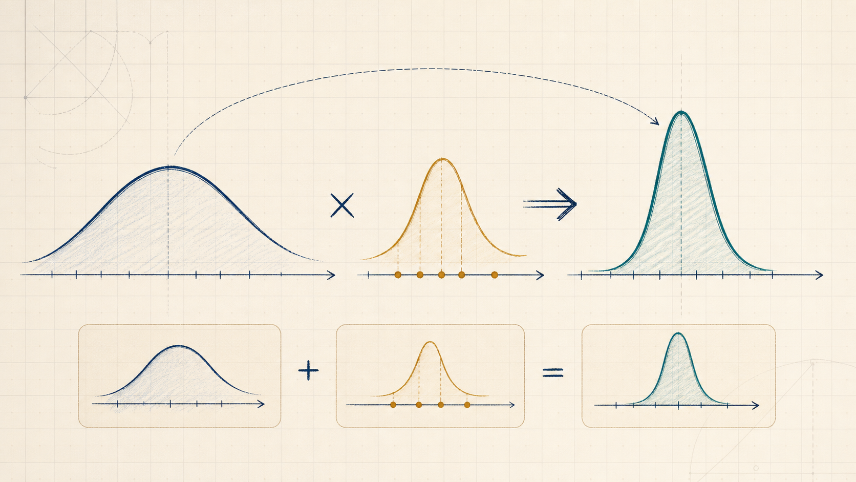
Bayesian inference updates a prior distribution over unknowns into a posterior by multiplying by the likelihood and normalizing.
Concept Structure
Bayesian Inference
01Intuition
Start with the picture, metaphor, or geometric mechanism.
02Math
Make the objects explicit and connect them with notation.
03Code
Mirror the equations with runnable implementation details.
04Interactive Demo
Manipulate the mechanism and watch the idea respond.
2prerequisites
1next concepts
2related links
Learning map
Bayesian InferenceBeforeDistributionsNow4/4 sections readyTryManipulate one control and predict the visible change.NextVariational Autoencoders
Conceptual Bridge
What should feel connected as you move through this page.
Bayesian inference updates a prior distribution over unknowns into a posterior by multiplying by the likelihood and normalizing.
The next edge should feel earned: use the demo prediction here before following Variational Autoencoders.
Test the linkManipulate one control and predict the visible change.Then continue to Variational Autoencoders
01IntuitionStart with the picture, metaphor, or geometric mechanism.02MathMake the objects explicit and connect them with notation.03CodeMirror the equations with runnable implementation details.04Interactive DemoManipulate the mechanism and watch the idea respond.
01
01
Intuition
Build the mental picture first so the rest of the page has something to attach to.
Section prompt
Maximum likelihood asks: which parameter makes the data look most probable?
Bayesian inference asks a different question: after seeing the data, what should we believe about each possible parameter?
That difference matters when data is scarce or uncertainty matters. The likelihood is a score of parameters by data fit. A prior is what you believed before the data. A posterior is the updated distribution after both forces are combined.
For a coin with unknown head probability , maximum likelihood might pick one number such as . Bayesian inference keeps a whole distribution over plausible values. With little data, the prior can still matter. With lots of data, and with a prior that gives nonzero density near the data-favored values, the likelihood usually concentrates the posterior near the parameters that explain the observations.
The mental model is not "Bayes is MLE plus vibes." It is a different object: MLE returns an estimate, while Bayesian inference returns a distribution over the unknown quantity.
02
02
Math
Translate the story into symbols, assumptions, and a derivation you can inspect.
Section prompt
Equation 1p(\theta\mid D)=\frac{p(D\mid\theta)p(\theta)}{p(D)}.Equation 2p(D)=\int p(D\mid\theta)p(\theta)\,d\theta
Let be an unknown parameter and let be observed data. Bayesian inference starts with a prior distribution or density and a likelihood . Bayes' rule gives the posterior:
For a continuous parameter, the denominator
is the evidence or marginal likelihood. Its job is to normalize the posterior so it integrates to .
If lives in a discrete set, replace the integral with a sum. The job is the same: add up prior-weighted likelihood over all possible parameter values.
For parameter comparison, the key proportional form is
This is the central contrast with maximum likelihood. The likelihood is a function of , but it is not automatically a probability distribution over . Multiplying by a prior and normalizing turns it into the posterior distribution.
For a coin with unknown head probability , suppose the data has heads and tails, with . The likelihood shape is
If records only the count of heads, the full binomial likelihood also has a factor . That factor does not depend on , so it disappears in proportional calculations.
If the prior is a beta distribution with ,
then
Multiplying prior and likelihood gives
so the posterior is
The maximum-likelihood estimate is
when . The posterior mean is
When , the posterior mean can also be written as
This is the clean bridge to maximum likelihood: the posterior mean is a weighted compromise between the prior mean and the MLE. The posterior distribution is the richer object; the mean is only one summary of it.
It is safe to think of as prior strength for this averaging formula. The density exponents are and , so pseudo-count language is only a mnemonic. The exact conjugate update is the parameter update .
03
03
Code
Keep the implementation aligned with the notation so the algorithm is legible.
Section prompt
import math
import numpy as np

def log_beta_fn(a, b):
    return math.lgamma(a) + math.lgamma(b) - math.lgamma(a + b)

def log_beta_pdf(theta, a, b):
    if theta <= 0 or theta >= 1:
        return -math.inf
    return (a - 1) * math.log(theta) + (b - 1) * math.log(1 - theta) - log_beta_fn(a, b)

alpha, beta = 2.0, 2.0
heads, tails = 8, 2

post_alpha = alpha + heads
post_beta = beta + tails
n = heads + tails

mle = None if n == 0 else heads / n
prior_mean = alpha / (alpha + beta)
posterior_mean = post_alpha / (post_alpha + post_beta)

print("MLE:", "undefined" if mle is None else round(mle, 3))
print("prior mean:", round(prior_mean, 3))
print("posterior mean:", round(posterior_mean, 3))
print("posterior:", f"Beta({post_alpha:.1f}, {post_beta:.1f})")

# Grid approximation to show prior * likelihood -> posterior shape.
grid = np.linspace(0.01, 0.99, 99)
log_prior = np.array([log_beta_pdf(theta, alpha, beta) for theta in grid])
log_likelihood = heads * np.log(grid) + tails * np.log(1 - grid)
log_unnormalized_posterior = log_prior + log_likelihood

# Normalize on the grid for inspection.
weights = np.exp(log_unnormalized_posterior - log_unnormalized_posterior.max())
weights = weights / weights.sum()
grid_mean = float(np.sum(grid * weights))

print("grid posterior mean approx:", round(grid_mean, 3))
The code mirrors the math: the prior is a density over , the likelihood scores the observed heads and tails for each , and the posterior beta parameters add the observed counts to the prior parameters.
04
04
Interactive Demo
Use direct manipulation to connect the explanation to a moving system.
Section prompt
Use the sliders and presets to compare prior strength against observed data. The prior and posterior curves are densities over . The likelihood curve is normalized only for display so its shape can be compared on the same plot.
Try the "strong prior, little data" preset, then the "data wins" preset. The MLE only follows the observed fraction. The posterior mean moves between prior belief and data fit, and the full posterior curve shows how much uncertainty remains.
Live Concept Demo
Explore Bayesian Inference
The stage is code-native and interactive. Use it to test the explanation against the mechanism.
difficulty 3/5undergraduatecode-aligned
Demo Prediction Checkpoint
Manipulate one control and predict the visible change.
Commit to what Bayesian Inference should make visible before reading the result.
After The First Pass
Turn the concept into an inspected object.
Once the invariant is visible in the intuition, math, code, and demo, use these panels to inspect the mechanism visually, check source support, practice the idea, and attach a grounded research question.
Mechanism Storyboard
See the idea move before the page explains it
Bayesian inference updates a prior distribution over unknowns into a posterior by multiplying by the likelihood and normalizing.
Prediction open01 / Intuition
Prediction lens
Start with the picture, metaphor, or geometric mechanism.
Commit first
Before reading further, choose the kind of change Bayesian Inference should make visible.
Visual Inquiry
Make the image answer a mathematical question
Bayesian inference updates a prior distribution over unknowns into a posterior by multiplying by the likelihood and normalizing.
4/4 stages readyLive demo connected
Visual cueWhich visible object should carry the first intuition?
Prediction
Which visible object should carry the first intuition?
Commit first
Pick the cue that should make Bayesian Inference easier to reason about before the page gives the answer.
Source Grounding
Canonical references for the mechanism on this page.
Grounds the probability notation and Bayes-rule prerequisites needed for the page.
Open sourceGrounds Bayesian inference as posterior updating under probabilistic models.
Open sourceClaim Review
Bayesian inference updates a prior distribution over unknowns into a posterior by multiplying by the likelihood and normalizing.
Claims without a substantive review badge still need exact source-support review.
deisenroth-2020-mml, murphy-2022-probabilistic-ml
Use equation, code, and demo objects to check whether the source support is operational.
Deisenroth et al. ground Bayes' rule as posterior = likelihood times prior divided by evidence and define evidence as the posterior normalizer; Murphy grounds Bayesian parameter inference as updating p(theta) with p(D|theta) and normalizing by marginal likelihood, while contrasting this with MLE as a point estimate.
Sources: Mathematics for Machine Learning, Probabilistic Machine Learning: An IntroductionChecks posterior updating and MLE contrast only; not approximate inference, hierarchy, asymptotics, posterior predictive decisions, or universal prior-strength advice. Code/demo are beta-Bernoulli witnesses; omitted binomial coefficients are theta-independent.A bounded review summary is present; still check caveats and exact source scope.MML supports Bayes-rule notation with prior, likelihood, evidence, and posterior labels, defines evidence/marginal likelihood as the normalizer, and notes that the full posterior retains more information than focusing on a maximum/statistic. Murphy directly supports parameter-level Bayesian updating as p(theta|D) proportional to p(theta)p(D|theta) normalized by p(D), contrasts this with MLE as a single likelihood-maximizing parameter estimate, and gives the beta-Bernoulli/binomial posterior update used by the page.
Reviewer: codex+oracle; reviewed 2026-05-07Practice Loop
Try the idea before it explains itself
Bayesian inference updates a prior distribution over unknowns into a posterior by multiplying by the likelihood and normalizing.
Readiness0/3 checks ready
Predict
Before touching the demo, predict one visible change that should happen in Bayesian Inference.
Hint 1
Reveal when your model needs a nudge.
Hint 2
Reveal when your model needs a nudge.
Hint 3
Reveal when your model needs a nudge.
Local checks
Claim
A concrete answer is on the canvas.
Mechanism
The answer names why the claim should hold.
Bridge
It touches the page context or a neighboring idea.
Object research drawerClose
ConceptBayesian InferenceProbability
Code witness comparisonBayesian Inference code witness 1if theta <= 0 or theta >= 1:Prediction before revealBayesian Inference interactive demoManipulate one control and predict the visible change.
Grounded room questionWhat is the smallest example that makes Bayesian Inference click without losing the math?Local snapshot ready
Research Room
Attach the question to an exact object
Pick the concept, equation, source, code witness, claim, misconception, or demo state before asking for help. The handoff stays grounded to that object.Open the draft below to save one note and next action in this browser.
Bayesian Inference
Anchored question
What is the smallest example that makes Bayesian Inference click without losing the math?
Local action draftNo local draft saved yetExpand only when ready to capture one local next action
Local action draft
This draft stays locally in this browser for concept:probability/bayesian-inference.
No local draft saved.
- Source ids to inspect: deisenroth-2020-mml, murphy-2022-probabilistic-ml
- Definition, prerequisite, and contrast concept links
- The equation or code witness that makes the concept operational
- One demo state that shows the invariant instead of a slogan
- The learner can state the mechanism in their own words
- The learner can name the prerequisite that would repair confusion
- The learner can predict how the mechanism changes under one perturbation
Grounded AI handoff
I am working in Continuous Function's research reading room. Object: concept - Bayesian Inference Object key: concept:probability/bayesian-inference Context: Probability Anchor id: concept/concept-notebook/probability/bayesian-inference Open question: What is the smallest example that makes Bayesian Inference click without losing the math? Evidence to inspect: - Source ids to inspect: deisenroth-2020-mml, murphy-2022-probabilistic-ml - Definition, prerequisite, and contrast concept links - The equation or code witness that makes the concept operational - One demo state that shows the invariant instead of a slogan What would resolve this: - The learner can state the mechanism in their own words - The learner can name the prerequisite that would repair confusion - The learner can predict how the mechanism changes under one perturbation Answer as a careful research tutor: stay source-grounded, separate verified evidence from assumptions, name the relevant math objects, and end with one next action.
concept/concept-notebook/probability/bayesian-inference
concept:probability/bayesian-inference