Variational Autoencoders

A latent-variable model trained by maximizing an evidence lower bound; the gap is KL(q_phi(z|x) || p_theta(z|x)), so the encoder is learned inference rather than just compression.

published · difficulty 4/5 · 20 min read

Intuition

Build the mental picture first so the rest of the page has something to attach to.

PredictName the object in plain language, then predict what should change.Leave with one reusable mental picture before notation appears.

Maximum likelihood asks for a model that assigns high log probability to the observed data:

\log p_\theta(x).

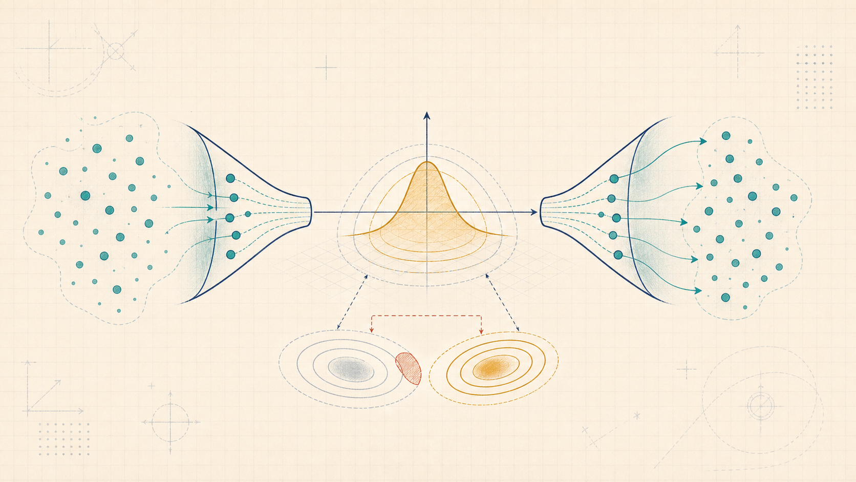
A variational autoencoder is a maximum-likelihood model with a hidden cause. It imagines that each observation $x$ was produced from an unobserved latent variable $z$ :

\begin{aligned} z &\sim p(z), \\ x &\sim p_\theta(x\mid z). \end{aligned}

Training would be easy if we could compute the marginal likelihood

\begin{aligned} p_\theta(x) &= \int p_\theta(x,z)\,dz. \end{aligned}

The problem is that this integral is usually hard for neural decoders. Bayesian inference tells us what we would like to use:

p_\theta(z\mid x).

But that posterior contains the same hard evidence term $p_\theta(x)$ . The VAE move is to learn an encoder

q_\phi(z\mid x)

that acts as a tractable approximate posterior.

The central mechanism is not "an autoencoder with noise." It is: replace the intractable posterior with a learned distribution $q_\phi(z\mid x)$ , then optimize a lower bound whose looseness is exactly a KL divergence from $q_\phi$ to the true posterior.

That is why VAEs sit at the intersection of maximum likelihood, Bayesian inference, and KL divergence.

Two natural next moves branch from this page. Normalizing flows ask what changes when the latent transformation is invertible and likelihood stays exact. Diffusion asks what changes when generation is learned as a gradual denoising process rather than as one sampled latent code.

Section prompt

Copy-only prompts — each action copies a page-grounded prompt to your clipboard. Nothing is sent by this site.

Math

Translate the story into symbols, assumptions, and a derivation you can inspect.

InspectTrack the same object through the notation and check each symbol.Leave with the invariant the equations preserve.

Equation 1Inspect equation objectp_\theta(x,z)=p(z)p_\theta(x\mid z); p_\theta(x)=\int p_\theta(x,z) dz; p_\theta(z\mid x)=(p_...Equation 2Inspect equation object\log p_\theta(x) = \mathcal L(\theta,\phi;x) + KL (q_\phi(z\mid x) \| p_\theta(z\mid x)); \ma...Equation 3Inspect equation object\mathbb E_q[\cdot] \equiv \mathbb E_{q(z)}[\cdot].

Latent variable likelihood

For one observed datapoint $x$ , assume a prior $p(z)$ and a decoder likelihood $p_\theta(x\mid z)$ . The latent-variable model, marginal likelihood, and true posterior are

\begin{aligned} p_\theta(x,z)&=p(z)p_\theta(x\mid z),\\ p_\theta(x)&=\int p_\theta(x,z)\,dz,\\ p_\theta(z\mid x)&=\frac{p_\theta(x,z)}{p_\theta(x)}. \end{aligned}

The evidence $p_\theta(x)$ appears in the denominator, so exact posterior inference and exact likelihood training are tied to the same difficult integral. The claim-bearing VAE move is summarized by

\begin{aligned} \log p_\theta(x) &= \mathcal L(\theta,\phi;x) + \mathrm{KL}\!\left(q_\phi(z\mid x)\,\|\,p_\theta(z\mid x)\right),\\ \mathcal L(\theta,\phi;x) &= \mathbb E_{q_\phi(z\mid x)}[\log p_\theta(x\mid z)] - \mathrm{KL}\!\left(q_\phi(z\mid x)\,\|\,p(z)\right),\\ \epsilon&\sim\mathcal N(0,I), \qquad z=\mu_\phi(x)+\sigma_\phi(x)\odot\epsilon. \end{aligned}

The first line says the ELBO gap is exactly the KL from the learned encoder $q_\phi(z\mid x)$ to the true posterior. The second line separates reconstruction likelihood from prior pressure. The third line keeps randomness in external noise $\epsilon$ , so gradients of sampled reconstruction terms can flow through $z$ into the encoder outputs.

The ELBO identity

Let $q_\phi(z\mid x)$ be any approximate posterior whose support is compatible with the true posterior. To keep the equations readable, write $q(z)$ for $q_\phi(z\mid x)$ and $\mathbb E_q$ for expectation under that distribution:

\mathbb E_q[\cdot] \equiv \mathbb E_{q(z)}[\cdot].

Using Bayes' rule and rearranging gives the exact identity

\log p_\theta(x)=\mathcal L+G.

Here $\mathcal L$ is the ELBO and $G$ is the inference gap. Let $p_*(z)$ denote the true posterior $p_\theta(z\mid x)$ . Then the gap is

G=\mathrm{KL}(q(z)\,\|\,p_*(z)).

Equivalently,

G=\mathbb E_q[\log q(z)-\log p_*(z)].

The ELBO term is

\mathcal L = \mathbb E_q[\log p_\theta(x,z)-\log q(z)].

The gap can also be read by subtraction:

G=\log p_\theta(x)-\mathcal L.

KL is nonnegative, so

\mathcal L(\theta,\phi;x)\le \log p_\theta(x).

Maximizing the ELBO improves this lower bound. The bound is tight exactly when the encoder distribution equals the true posterior, up to probability-zero events.

Reconstruction likelihood plus prior KL

Because

\log p_\theta(x,z) = \log p_\theta(x\mid z)+\log p(z),

the ELBO can be rewritten as

\begin{aligned} \mathcal L &= \mathbb E_q[\log p_\theta(x\mid z)] \\ &\quad- \mathrm{KL}(q(z)\,\|\,p(z)). \end{aligned}

The first term is a reconstruction log likelihood, not generically a pixel distance. The second term keeps the encoder's posterior close to the prior used for generation. At generation time we sample $z\sim p(z)$ , not $z\sim q_\phi(z\mid x)$ for a training example, so the prior match is load-bearing.

Reconstruction likelihood is not always MSE

The reconstruction term is

\mathbb E_q[\log p_\theta(x\mid z)].

It becomes a familiar loss only after choosing a decoder distribution. With a fixed-variance Gaussian decoder centered at $f_\theta(z)$ , the negative log likelihood is a scaled squared error plus a constant. So MSE appears as a Gaussian negative log likelihood only after that modeling choice.

If $x$ is binary and

p_\theta(x\mid z)=\operatorname{Bernoulli}(\pi_\theta(z)),

then the negative reconstruction log likelihood is binary cross-entropy.

Reparameterization trick

For a diagonal Gaussian encoder, the network outputs $\mu_\phi(x)$ and $\sigma_\phi(x)$ . We sample with external noise:

\epsilon\sim\mathcal N(0,I), \qquad z=\mu_\phi(x)+\sigma_\phi(x)\odot\epsilon.

This keeps the randomness in $\epsilon$ and makes the sample differentiable with respect to the encoder outputs $\mu_\phi(x)$ and $\sigma_\phi(x)$ .

Beta-VAE objective

A beta-VAE changes the training objective to

\begin{aligned} \mathcal L_\beta &= \mathbb E_q[\log p_\theta(x\mid z)] \\ &\quad- \beta\,\mathrm{KL}(q(z)\,\|\,p(z)). \end{aligned}

When $\beta=1$ , this is the standard VAE ELBO. When $\beta\ne 1$ , it is a modified objective rather than the original ELBO. For $\beta>1$ , it remains a lower bound because it subtracts extra nonnegative KL penalty, but it is no longer the standard maximum-likelihood ELBO. For $\beta<1$ , it is generally not guaranteed to lower-bound $\log p_\theta(x)$ .

Larger $\beta$ puts more pressure on $z$ to carry less information and stay close to the prior. This can encourage more factor-like representations in some settings, but it does not guarantee disentanglement. If the pressure is too strong, the encoder may approach $q_\phi(z\mid x)\approx p(z)$ , so $z$ carries little information about $x$ .

Section prompt

Copy-only prompts — each action copies a page-grounded prompt to your clipboard. Nothing is sent by this site.

Code

Keep the implementation aligned with the notation so the algorithm is legible.

TraceMatch variables to symbols before reading the implementation.Leave with a runnable witness for the math.

Code witness 1import math def log_norm(x, mean, var): return -0.5 * (math.log(2 * math.pi * var) + (x - mea...python

This scalar linear-Gaussian example is small enough that we can compute the exact marginal likelihood, exact posterior, ELBO, and inference gap, then check a one-sample reparameterized reconstruction gradient by finite differences.

import math

def log_norm(x, mean, var):
    return -0.5 * (math.log(2 * math.pi * var) + (x - mean) ** 2 / var)

def kl_norm(mu0, var0, mu1, var1):
    return 0.5 * (var0 / var1 + (mu1 - mu0) ** 2 / var1 - 1 + math.log(var1 / var0))

x, w, b, sigma_x = 1.5, 1.2, -0.1, 0.3  # z~N(0,1), x|z~N(wz+b,sigma_x^2)
var_x = sigma_x ** 2
mu_q, logvar_q = 0.3, -0.7              # q(z|x)=N(mu_q, exp(logvar_q))
var_q = math.exp(logvar_q)

log_px = log_norm(x, b, w * w + var_x)
post_var = 1 / (1 + w * w / var_x)
post_mu = post_var * w * (x - b) / var_x
recon = -0.5 * (math.log(2 * math.pi * var_x) + ((x - b - w * mu_q) ** 2 + w * w * var_q) / var_x)
kl_prior = kl_norm(mu_q, var_q, 0, 1)
elbo = recon - kl_prior
gap = log_px - elbo
kl_post = kl_norm(mu_q, var_q, post_mu, post_var)
assert abs(gap - kl_post) < 1e-10

eps = -0.4
def sampled_recon(mu, logvar):
    sigma = math.exp(0.5 * logvar)
    z = mu + sigma * eps
    return log_norm(x, w * z + b, var_x), z, sigma

sample_loglik, z, sigma = sampled_recon(mu_q, logvar_q)
dloglik_dz = (x - (w * z + b)) * w / var_x
path_mu = dloglik_dz
path_logvar = dloglik_dz * 0.5 * sigma * eps
h = 1e-5
fd_mu = (sampled_recon(mu_q + h, logvar_q)[0] - sampled_recon(mu_q - h, logvar_q)[0]) / (2 * h)
fd_logvar = (sampled_recon(mu_q, logvar_q + h)[0] - sampled_recon(mu_q, logvar_q - h)[0]) / (2 * h)
assert abs(path_mu - fd_mu) < 1e-7
assert abs(path_logvar - fd_logvar) < 1e-7

print(round(elbo, 3), round(log_px, 3), round(gap, 3), round(sample_loglik, 3))

For a batched neural VAE, typical shapes are:

x: (B, D)
encoder outputs mu, logvar: (B, K)
noise eps: (S, B, K)
latent samples z = mu[None, :, :] + exp(0.5 * logvar)[None, :, :] * eps: (S, B, K)
decoder log likelihood per sample: (S, B)
Monte Carlo reconstruction estimate: (B,)
analytic diagonal-Gaussian KL: (B,)
per-example ELBO: (B,)
optimization loss -elbo.mean(): scalar

Section prompt

Copy-only prompts — each action copies a page-grounded prompt to your clipboard. Nothing is sent by this site.

Interactive Demo

Use direct manipulation to connect the explanation to a moving system.

ManipulateChange one control and predict the visible response before reveal.Leave with the observed invariant or a repaired model.

Live Concept Demo

Explore Variational Autoencoders

The stage is code-native and interactive. Use it to test the explanation against the mechanism.

difficulty 4/5undergraduatecode-aligned

Demo inquiry checkpoint

Manipulate one control and predict the visible change.

01Choose lensTrace a quantity

02ObserveDemo state pending

03GroundName the equation, invariant, or control that explains it.

04CarryNext: Normalizing Flows: Tractable Density via Invertible Transforms

Choose what to inspect in Variational Autoencoders. This shared fallback is an observation guide, not evidence of learning.

Loading interactive demo...

The demo keeps the latent variable one-dimensional so the hidden inference geometry can be revealed after a prediction. Move the approximate posterior $q(z\mid x)$ , inspect the prior and likelihood shape, then predict what the ELBO gap will diagnose.

After reveal, compare the target curve and identity values with your prediction. The point is to feel the ELBO as a lower bound whose looseness is measured by the mismatch between $q$ and the hidden target distribution.

Section prompt

Copy-only prompts — each action copies a page-grounded prompt to your clipboard. Nothing is sent by this site.

Object

4/4 sections ready

Concept: Variational Autoencoders

What is the smallest example that makes Variational Autoencoders click without losing the math?

BeforeMaximum LikelihoodNow4/4 sections readyTryManipulate one control and predict the visible change.NextNormalizing Flows: Tractable Density via Invertible Transforms

Object contextGenerative Models

StateGenerative Models

2 sources attachedChecking local snapshot

concept:generative-models/vaes

Math3 equation objectsp_\theta(x,z)=p(z)p_\theta(x\mid z); p_\theta(x)=\int p_\theta(x,z) dz; p_\theta(z\mid x)=(p_...CodeVariational Autoencoders code witness 1assert abs(gap - kl_post) < 1e-10 DemoVariational Autoencoders predictionManipulate one control and predict the visible change.

ConceptLearner lens

Variational Autoencoders

What is the smallest example that makes Variational Autoencoders click without losing the math?

Mode questionCan I say the mechanism back in one sentence before I reveal anything?

Start with the prediction checkpoint, then compare the reveal to the mental model.

Take this move

Study modes

Keep the object fixed; change the lens.

01PredictCommit before reveal.02ExplainName the invariant.03Ground2 source links nearby.04ExperimentChange one knob.05CarrySave the next question.

Route back through the notebook

Carry the same object through intuition, math, code, and demo.

4/4 sections ready

Carry inMaximum Likelihood

Bring the mental model from Maximum Likelihood; this page will reuse it instead of restarting from zero.

Work hereVariational Autoencoders

A latent-variable model trained by maximizing an evidence lower bound; the gap is KL(q_phi(z|x) || p_theta(z|x)), so the encoder is learned inference rather than just compression.

Carry outNormalizing Flows: Tractable Density via Invertible Transforms

The next edge should feel earned: use the demo prediction here before following Normalizing Flows: Tractable Density via Invertible Transforms.

After The First Pass

Turn the concept into an inspected object.

The lower panels are one second act: keep the object fixed, inspect it visually, check source boundaries, practice transfer, then attach the research question.

ConceptVariational AutoencodersGenerative Models

01MechanismInspect motionSee how the idea changes form before adding more explanation.02VisualChoose a cueBind one visible mark to one mathematical role.03SourcesCheck boundary2 source links attached to the object.04ClaimAudit evidenceTreat the page claim as something to verify.05PracticeAttempt transferWrite before feedback so the model has something to repair.06RoomAsk groundedAttach the question to the same exact object.

Mechanism Storyboard

See the idea move before the page explains it

A latent-variable model trained by maximizing an evidence lower bound; the gap is KL(q_phi(z|x) || p_theta(z|x)), so the encoder is learned inference rather than just compression.

Demo notes open01 / Intuition

Editorial generative-model illustration of data encoded into a latent distribution and decoded back into reconstructed samples.

Prediction lens

Start with the picture, metaphor, or geometric mechanism.

Commit first

Before reading further, choose the kind of change Variational Autoencoders should make visible.

Visual Inquiry

Make the image answer a mathematical question

A latent-variable model trained by maximizing an evidence lower bound; the gap is KL(q_phi(z|x) || p_theta(z|x)), so the encoder is learned inference rather than just compression.

4/4 stages readyDemo notes connected

Visual cueWhich visible object should carry the first intuition?

Inspection depth2/4

Prediction

Which visible object should carry the first intuition?

Commit first

Pick the cue that should make Variational Autoencoders easier to reason about before the page gives the answer.

Source Grounding

Canonical references for the mechanism on this page.

Object - ConceptVariational AutoencodersQuestion

What is the smallest example that makes Variational Autoencoders click without losing the math?

concept:generative-models/vaes

Boundary

sources: kingma-2013-auto-encoding-variational-bayes, rezende-2014-stochastic-backprop

Check

Open the closest source note before trusting the local explanation.

Evidence

2 selected-object sources shown first; 2 references total.

Next move

Audit the claim boundary, then ask from the same selected object.

selected object source · paper · 2013Auto-Encoding Variational BayesKingma and Welling

Located CF editorial boundary

Introduces the reparameterized VAE objective and the evidence lower bound training view.

Used here as

Kingma/Welling and Rezende/Mohamed/Wierstra both ground VAEs/deep latent-variable models in ELBO optimization with learned inference networks and reparameterized or stochastic backpropaga...

Caveat

The reconstruction term is an expectation under q_phi and often Monte Carlo estimated. Pathwise gradients require a differentiable transform of parameter-independent noise, so this does n...

Open source

selected object source · paper · 2014Stochastic Backpropagation and Approximate Inference in Deep Generative ModelsRezende, Mohamed, and Wierstra

Located CF editorial boundary

Grounds stochastic backpropagation for latent-variable generative models with learned inference networks.

Used here as

Kingma/Welling and Rezende/Mohamed/Wierstra both ground VAEs/deep latent-variable models in ELBO optimization with learned inference networks and reparameterized or stochastic backpropaga...

Caveat

The reconstruction term is an expectation under q_phi and often Monte Carlo estimated. Pathwise gradients require a differentiable transform of parameter-independent noise, so this does n...

Open source

Claim Review

A latent-variable model trained by maximizing an evidence lower bound; the gap is KL(q_phi(z|x) || p_theta(z|x)), so the encoder is learned inference rather than just compression.

Object - ConceptVariational AutoencodersQuestion

What is the smallest example that makes Variational Autoencoders click without losing the math?

concept:generative-models/vaes

Boundary

sources: kingma-2013-auto-encoding-variational-bayes, rezende-2014-stochastic-backprop

Check

Treat every claim as provisional until source support and a local witness agree.

Evidence

1 structured claim check on this concept.

Next move

Run the prediction or practice transfer before asking for a grounded review.

1 CF editorial source-scope review recorded

Publisher-side editorial review is not independent replication. Claims without it still need exact source-support review. 2 references and 3 local witnesses are available for inspection.

A VAE fits a latent-variable generative model by maximizing the ELBO: q_phi(z|x) approximates the usually intractable posterior, E_q[log p_theta(x|z)] rewards reconstruction likelihood, KL(q_phi(z|x)||p(z)) penalizes deviation from the prior, and reparameterization gives pathwise gradients through z samples.

Registered CF editorial boundary

Auto-Encoding Variational BayesIntroduces the reparameterized VAE objective and the evidence lower bound training view.Stochastic Backpropagation and Approximate Inference in Deep Generative ModelsGrounds stochastic backpropagation for latent-variable generative models with learned inference networks.

Used here as

Kingma/Welling and Rezende/Mohamed/Wierstra both ground VAEs/deep latent-variable models in ELBO optimization with learned inference networks and reparameterized or stochastic backpropagation estimators. Loc...

Local witness

source-span-kingma-2013-auto-encoding-variational-bayes source-span-rezende-2014-stochastic-backprop math-object-1 math-object-2 code-witness-1 interactive-demo

Equation 1

\begin{aligned} p_\theta(x,z)&=p(z)p_\theta(x\mid z),\\ p_\theta(x)&=\int p_\theta(x,z)\,dz,\\ p_\theta(z\mid x)&=\frac{p_\theta(x,z)}{p_\theta(x)}. \end{aligned}

Equation 2

\begin{aligned} \log p_\theta(x) &= \mathcal L(\theta,\phi;x) + \mathrm{KL}\!\left(q_\phi(z\mid x)\,\|\,p_\theta(z\mid x)\right),\\ \mathcal L(\theta,\phi;x) &= \mathbb E_{q_\phi(z\mid x)}[\log p_\theta(x\mid z)] - \mathrm{KL}\!\left(q_\phi(z\mid x)\,\|\,p(z)\right),\\ \epsilon&\sim\mathcal N(0,I), \qquad z=\mu_\phi(x)+\sigma_\phi(x)\odot\epsilon. \end{aligned}

Caveat

The reconstruction term is an expectation under q_phi and often Monte Carlo estimated. Pathwise gradients require a differentiable transform of parameter-independent noise, so this does not cover discrete or...

Review stateCF editorial source-scope reviewClaim metadata: source checkedPublisher-side editorial review only; not independent replication. Check caveats and exact source scope.

Kingma/Welling support q_phi(z|x) as a learned recognition model for the intractable posterior, derive log p_theta(x)=ELBO+KL(q||posterior), decompose the ELBO into E_q log p_theta(x|z)-KL(q||p(z)), and give Gaussian reparameterization. Rezende et al. independently support the recognition-model, lower-bound/free-energy, reconstruction/regularization, and stochastic-backprop structure. Local math, code, and demo now witness the ELBO gap, prior KL, reparameterized sample, and prediction-gated posterior diagnostics.

Reviewer: codex+oracle+codex-5.3; reviewed 2026-05-08

Practice notebook

Use the idea, then test it somewhere new

A latent-variable model trained by maximizing an evidence lower bound; the gap is KL(q_phi(z|x) || p_theta(z|x)), so the encoder is learned inference rather than just compression.

AttemptNo learning claim inferred

Object - ConceptVariational AutoencodersQuestion

What is the smallest example that makes Variational Autoencoders click without losing the math?

concept:generative-models/vaes

Boundary

sources: kingma-2013-auto-encoding-variational-bayes, rezende-2014-stochastic-backprop

Check

Use one state from Variational Autoencoders to explain what changes, why it changes, and which assumption the explanation needs.

Evidence

No learner move yet; no learning state is inferred.

Next move

Write first, use only the help you need, then try a new case without it.

Explain

Use one state from Variational Autoencoders to explain what changes, why it changes, and which assumption the explanation needs.

Hint 1

Reveal when your model needs a nudge.

Hint 2

Reveal when your model needs a nudge.

Hint 3

Reveal when your model needs a nudge.

Your answer canvas

Attempt context

Learner move

Write an attempt before asking the companion.

Assistance used

0 of 3 progressive hints opened.

Evidence boundary

This draft and any AI response do not establish mastery; a later unassisted case can.

Misconception check

Grounded object roomClose

Selected object routeAsk from this object; carry one invariant back.sources: kingma-2013-auto-encoding-variational-bayes, rezende-2014-stochastic-backprop

ObjectConceptVariational Autoencoders
PredictBefore revealVariational Autoencoders prediction
WitnessCompare codeVariational Autoencoders code witness 1
RoomAsk groundedChecking local snapshot

ConceptVariational AutoencodersGenerative Models

Code witness comparisonVariational Autoencoders code witness 1assert abs(gap - kl_post) < 1e-10 Prediction before revealVariational Autoencoders predictionManipulate one control and predict the visible change.

Grounded room questionWhat is the smallest example that makes Variational Autoencoders click without losing the math?Checking local snapshot

Research Room

Attach the question to an exact object

Pick the concept, equation, source, code witness, claim, misconception, or demo state before asking for help. The handoff stays grounded to that object.

Next local actionNo local draft saved yet

Open the draft below to save one note and next action in this browser.

conceptGenerative Models

Variational Autoencoders

Anchored question

What is the smallest example that makes Variational Autoencoders click without losing the math?

Source boundaryInspect source ids: kingma-2013-auto-encoding-variational-bayes, rezende-2014-stochastic-backpropStable content-object key attached

Role lenses for this object

These are fixed, deterministic perspectives derived from the selected object. They do not represent people, community contributions, or independent review.

Learner evidence requestAsk what would make "Variational Autoencoders" feel predictable rather than familiar.

Assumption

Source ids kingma-2013-auto-encoding-variational-bayes, rezende-2014-stochastic-backprop must support the exact object, not just the surrounding topic.

Source-checking summary

Treat this as a mechanism object: connect the definition to one equation, code witness, or demo before broadening the discussion.

Proposed experiment

Ask the learner to perturb one representation, then check whether the same invariant survives in math, code, and demo.

Next action

The learner can state the mechanism in their own words

Evidence4 checks

PredictionChecking carried observation

ActionReady for one action

AILearner handoff ready

Open source object

01PredictionChecking browser-local route memory

02EvidenceChecking for a carried observation

03BoundaryInspect source ids: kingma-2013-auto-encoding-variational-bayes, rezende-2014-stochastic-backprop

04Next moveSave one next action

Local action draftNo local draft saved yetExpand only when ready to capture one local next action

Local action draft

This draft stays locally in this browser for concept:generative-models/vaes.

Draft noteNext action

No local draft saved.

Evidence to inspect

Source ids to inspect: kingma-2013-auto-encoding-variational-bayes, rezende-2014-stochastic-backprop
Definition, prerequisite, and contrast concept links
The equation or code witness that makes the concept operational
One demo state that shows the invariant instead of a slogan

What would resolve this

The learner can state the mechanism in their own words
The learner can name the prerequisite that would repair confusion
The learner can predict how the mechanism changes under one perturbation

Object-attached AI handoff

I am working in Continuous Function's research reading room. Object: concept - Variational Autoencoders Object key: concept:generative-models/vaes Context: Generative Models Anchor id: concept/concept-notebook/generative-models/vaes Open question: What is the smallest example that makes Variational Autoencoders click without losing the math? Evidence to inspect: - Source ids to inspect: kingma-2013-auto-encoding-variational-bayes, rezende-2014-stochastic-backprop - Definition, prerequisite, and contrast concept links - The equation or code witness that makes the concept operational - One demo state that shows the invariant instead of a slogan Deterministic role lenses for this object: - Boundary: fixed perspectives, not people, community contributions, or independent review - Source-checking summary: Treat this as a mechanism object: connect the definition to one equation, code witness, or demo before broadening the discussion. - Proposed experiment: Ask the learner to perturb one representation, then check whether the same invariant survives in math, code, and demo. - Teach/transfer move: Turn the mechanism into one sentence that predicts a neighboring concept. - Assumptions: - Source ids kingma-2013-auto-encoding-variational-bayes, rezende-2014-stochastic-backprop must support the exact object, not just the surrounding topic. - The stable content-object key lets local drafts, prompts, and route memory attach without changing the source page. - The concept explanation is local atlas prose until checked against its math, code, and source support. - Prerequisite gaps should become a repair route, not a reason to leave the object vague. - Role-lens requests: - Learner: ask for "Ask what would make "Variational Autoencoders" feel predictable rather than familiar." | assumption: Source ids kingma-2013-auto-encoding-variational-bayes, rezende-2014-stochastic-backprop must support the exact object, not just the surrounding topic. | next action: The learner can state the mechanism in their own words - Researcher: ask for "Source ids to inspect: kingma-2013-auto-encoding-variational-bayes, rezende-2014-stochastic-backprop" | assumption: The stable content-object key lets local drafts, prompts, and route memory attach without changing the source page. | next action: The learner can name the prerequisite that would repair confusion - Experimenter: ask for "Choose one variable or condition to perturb before asking for an explanation." | assumption: The concept explanation is local atlas prose until checked against its math, code, and source support. | next action: The learner can predict how the mechanism changes under one perturbation - Professor: ask for "Find the smallest transferable rule a learner could reuse without the AI." | assumption: Prerequisite gaps should become a repair route, not a reason to leave the object vague. | next action: Teach or transfer: Turn the mechanism into one sentence that predicts a neighboring concept. What would resolve this: - The learner can state the mechanism in their own words - The learner can name the prerequisite that would repair confusion - The learner can predict how the mechanism changes under one perturbation Answer as a careful research tutor: stay source-grounded, separate verified evidence from assumptions, name the relevant math objects, and end with one next action. Current deterministic role lens for this object: - Role lens: Learner - Evidence request: Ask what would make "Variational Autoencoders" feel predictable rather than familiar. - Assumption to keep visible: Source ids kingma-2013-auto-encoding-variational-bayes, rezende-2014-stochastic-backprop must support the exact object, not just the surrounding topic. - Proposed experiment: Ask the learner to perturb one representation, then check whether the same invariant survives in math, code, and demo. - Next action: The learner can state the mechanism in their own words

concept/concept-notebook/generative-models/vaes
concept:generative-models/vaes

Learning Map

Before / Now / Try / Next

BeforeMaximum Likelihood

NowIntuition → Math → Code → Demo

TryManipulate one control and predict the visible change.

NextNormalizing Flows: Tractable Density via Invertible Transforms

Learnerpicture first Researchersource check Experimentertest the demo Professorname invariant

01Predict 02Ground 03Code 04Carry

01Intuitionready
02Mathready
03Codeready
04Interactive Demoready

Object Companion

Ask beside the selected object

A latent-variable model trained by maximizing an evidence lower bound; the gap is KL(q_phi(z|x) || p_theta(z|x)), so the encoder is learned inference rather than just compression.

Your question

GoalComfortStyleStuck on

Context prompt

You are my AI learning companion for Continuous Function. Current context: Generative Models concept. Learning surface: Variational Autoencoders. What this page says: A latent-variable model trained by maximizing an evidence lower bound; the gap is KL(q_phi(z|x) || p_theta(z|x)), so the encoder is learned inference rather than just compression. Current section: Intuition, math, code, and interactive demo. Suggested next step: Manipulate one control and predict the visible change.. Learner goal: Understand the idea. Learner comfort level: New to this. Preferred explanation style: Visual first. Task: Explain the central idea in plain language, then restate it with the exact math objects from the page. Answer in a way that helps me learn: ask one clarifying question only if needed, use intuition before notation, and end with one thing I should try on the page.

Copy-only tool: this panel composes a prompt for an AI tool you already use. Nothing you enter here is sent from this page.

Domain

Generative Models

generative-modelsvaevariational-inferenceelbokl-divergence

Prerequisites

Maximum Likelihood Bayesian Inference KL Divergence (Relative Entropy)

Leads To

Normalizing Flows: Tractable Density via Invertible Transforms Diffusion, Score-Based Models & Flow Matching

Score Matching & Score-Based Generative Models

Within this domain