Maximum Likelihood

Maximum likelihood fits parameters by making the observed data most probable; for classifiers it becomes negative log-likelihood, cross-entropy, and a KL fit to the empirical distribution.

published · difficulty 3/5 · 18 min read

Reading map and next steps

Intuition

Build the mental picture first so the rest of the page has something to attach to.

PredictName the object in plain language, then predict what should change.Leave with one reusable mental picture before notation appears.

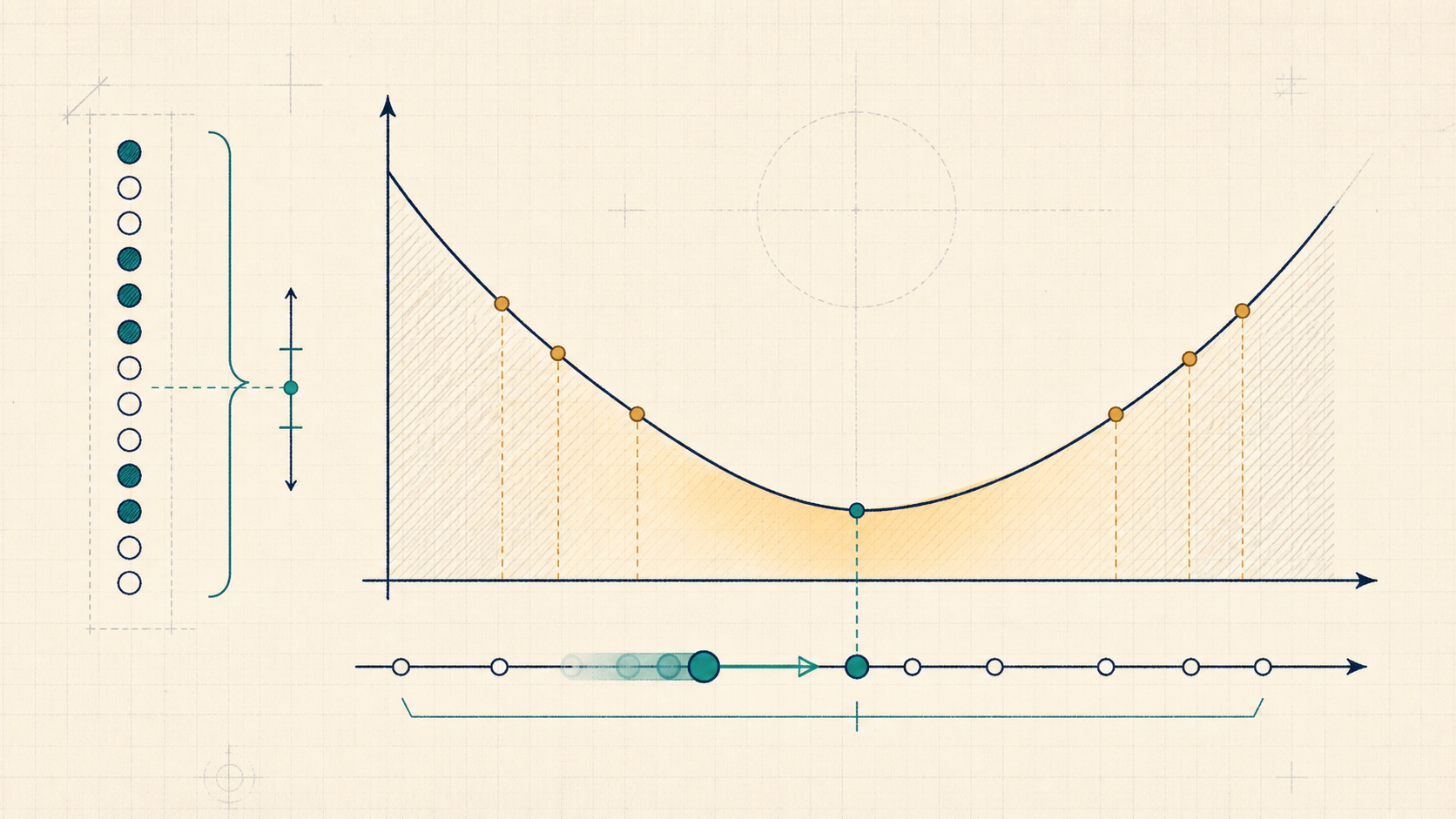
You observed data. Among all parameter settings your model allows, which one makes that exact data look least surprising?

Maximum likelihood answers by holding the observations fixed and moving the model parameters. A parameter setting is good when it assigns high probability, or high density for continuous data, to the values that actually appeared.

For a biased coin, if you saw 14 heads in 20 flips, the most likely head probability is not found by asking which coin is "fair." It is found by asking which value of $\theta$ makes the sequence with 14 heads and 6 tails most plausible. The answer is $\hat\theta=14/20$ .

This same idea scales into deep learning. A classifier assigns probabilities to labels. A language model assigns probabilities to next tokens. Training by maximum likelihood means increasing the probability assigned to the observed labels or tokens. The negative log of that likelihood is the loss the optimizer actually minimizes.

The analogy has one important limit: likelihood is a score of parameters after the data are fixed. It is not, by itself, a posterior probability that a parameter is true. Bayesian inference adds a prior and normalizes over parameter values; maximum likelihood just finds the parameter value with the highest data score.

Section prompt

Copy-only prompts — each action copies a page-grounded prompt to your clipboard. Nothing is sent by this site.

Math

Translate the story into symbols, assumptions, and a derivation you can inspect.

InspectTrack the same object through the notation and check each symbol.Leave with the invariant the equations preserve.

Equation 1Inspect equation objectL(\theta)=\prod_{i=1}^n p_\theta(x_i).Equation 2Inspect equation object\ell(\theta)=\log L(\theta)=\sum_{i=1}^n \log p_\theta(x_i).Equation 3Inspect equation object\mathcal L_{NLL}(\theta)=-(1)/(n)\sum_{i=1}^n \log p_\theta(x_i).

Let $X_1,\dots,X_n$ be observed values treated as independent draws from a fixed parametric model family $p_\theta(x)$ . The model family and parameter space are chosen before fitting; maximum likelihood only moves $\theta$ inside that family. All logarithms below are natural logarithms, so losses are measured in nats.

The likelihood is a function of the parameter:

L(\theta)=\prod_{i=1}^n p_\theta(x_i).

The data values are fixed inside this expression. The variable being optimized is $\theta$ . Because products of many probabilities become tiny, we usually maximize log likelihood:

\ell(\theta)=\log L(\theta)=\sum_{i=1}^n \log p_\theta(x_i).

Equivalently, training minimizes average negative log-likelihood:

\mathcal L_{\mathrm{NLL}}(\theta)=-\frac{1}{n}\sum_{i=1}^n \log p_\theta(x_i).

For a Bernoulli model with $x_i\in\{0,1\}$ , parameter space $\theta\in[0,1]$ , and $P_\theta(X=1)=\theta$ , suppose $s$ observations are $1$ and $f=n-s$ are $0$ . For an ordered sequence,

L(\theta)=\theta^s(1-\theta)^f,

and

\ell(\theta)=s\log\theta+f\log(1-\theta).

If the data record only the count $s$ rather than the ordered sequence, the likelihood also has a binomial coefficient $\binom n s$ . That factor does not depend on $\theta$ , so it does not change the MLE.

On the open interval $0<\theta<1$ , the derivative is

\frac{d\ell}{d\theta}=\frac{s}{\theta}-\frac{f}{1-\theta}.

When $0<s<n$ , setting it to zero gives

\hat\theta_{\mathrm{MLE}}=\frac{s}{n}.

When $s=0$ or $s=n$ , there is no interior critical point. On the closed interval $[0,1]$ , the MLE is the boundary value $\hat\theta_{\mathrm{MLE}}=0$ or $\hat\theta_{\mathrm{MLE}}=1$ . On the open interval $(0,1)$ , the maximum is not attained; the likelihood only approaches its supremum at the boundary. The demo displays $\theta\in[0.01,0.99]$ to avoid infinities from $\log 0$ .

This is not a coincidence. The MLE for this Bernoulli family is the empirical frequency because the best one-parameter Bernoulli distribution matches the observed mass on $1$ and $0$ .

Now write the empirical distribution as

\hat p(1)=\frac{s}{n},\qquad \hat p(0)=\frac{f}{n}.

In this finite discrete setting, the average NLL is the cross-entropy from the empirical distribution to the model distribution:

\mathcal L_{\mathrm{NLL}}(\theta)=H(\hat p,p_\theta).

H(\hat p,p_\theta)=-\sum_{x\in\{0,1\}}\hat p(x)\log p_\theta(x).

And cross-entropy decomposes as

H(\hat p,p_\theta)=H(\hat p)+\mathrm{KL}(\hat p\|p_\theta).

Here the empirical entropy is

H(\hat p)=-\sum_x \hat p(x)\log\hat p(x),

and the forward KL mismatch is

\mathrm{KL}(\hat p\|p_\theta)=\sum_x \hat p(x)\log\frac{\hat p(x)}{p_\theta(x)}.

The sums are over $x\in\{0,1\}$ . Terms with $\hat p(x)=0$ contribute $0$ . If $\hat p(x)>0$ but $p_\theta(x)=0$ , the NLL and KL are infinite.

Since $H(\hat p)$ does not depend on $\theta$ , maximum likelihood is equivalent here to minimizing the KL mismatch. If the model family cannot represent the empirical distribution exactly, MLE chooses the member of the family with the smallest mismatch inside that family.

The derivative of the average Bernoulli NLL with respect to $\theta$ is

\frac{d\mathcal L}{d\theta}=-\frac{\hat p}{\theta}+\frac{1-\hat p}{1-\theta}.

If $\theta$ is produced by a logit $a$ with $\theta=\sigma(a)$ , then the chain rule gives

\frac{d\mathcal L}{da}=\theta-\hat p.

The demo reports this logit gradient. It is not the slope of the plotted curve with respect to $\theta$ .

For neural classifiers, $p_\theta(y\mid x)$ is conditional on the input. The dataset objective is

-\frac{1}{n}\sum_{i=1}^n \log p_\theta(y_i\mid x_i).

For language models, $y_i$ is the next token at a position. The mechanism is the same: assign high probability to observed data, take logs, average, then use gradients to move parameters.

For continuous models, $p_\theta(x)$ is a density rather than a probability mass. The likelihood scores density at the observed points; the probability of any exact point can be zero even while the likelihood density is high. Likelihood comparisons are meaningful within the same model and measurement units. The finite-sample objective is an empirical average of log density; a KL interpretation is clean when comparing expected NLL under a data-generating density to model densities with respect to the same base measure.

Section prompt

Copy-only prompts — each action copies a page-grounded prompt to your clipboard. Nothing is sent by this site.

Code

Keep the implementation aligned with the notation so the algorithm is legible.

TraceMatch variables to symbols before reading the implementation.Leave with a runnable witness for the math.

Code witness 1import numpy as np # Observed Bernoulli data: 1=head/success, 0=tail/failure. # Shape: y is (...python

import numpy as np

# Observed Bernoulli data: 1=head/success, 0=tail/failure.
# Shape: y is (n,), theta is a scalar.
y = np.array([1, 1, 0, 1, 1, 0, 1, 0, 1, 1,
              1, 0, 1, 1, 0, 1, 0, 1, 1, 1])

n = y.size
s = int(y.sum())
f = n - s
p_hat = s / n

def bernoulli_nll(theta):
    theta = np.clip(theta, 1e-12, 1 - 1e-12)
    return float(-(s * np.log(theta) + f * np.log(1 - theta)) / n)

def binary_entropy(p):
    return float(sum(-value * np.log(value) for value in [p, 1 - p] if value > 0))

def bernoulli_kl(p, theta):
    theta = np.clip(theta, 1e-12, 1 - 1e-12)
    out = 0.0
    if p > 0:
        out += p * (np.log(p) - np.log(theta))
    if p < 1:
        out += (1 - p) * (np.log(1 - p) - np.log(1 - theta))
    return float(out)

grid = np.linspace(0.01, 0.99, 99)
theta_grid_mle = grid[np.argmin([bernoulli_nll(t) for t in grid])]

# Closed-form MLE for Bernoulli.
theta_mle = p_hat

empirical_entropy = binary_entropy(p_hat)
kl_at_theta_04 = bernoulli_kl(p_hat, 0.4)

assert abs(bernoulli_nll(0.4) - (empirical_entropy + kl_at_theta_04)) < 1e-12

print("successes / n:", s, "/", n)
print("empirical p_hat:", round(p_hat, 3))
print("closed-form MLE:", round(theta_mle, 3))
print("grid MLE:", round(theta_grid_mle, 3))
print("NLL at theta=0.4:", round(bernoulli_nll(0.4), 3))
print("H(p_hat):", round(empirical_entropy, 3))
print("KL(p_hat || theta=0.4):", round(kl_at_theta_04, 3))

The code mirrors the math: the observations determine the empirical distribution, the likelihood is a function of $\theta$ , and the minimum average NLL occurs at $\theta=\hat p$ .

Section prompt

Copy-only prompts — each action copies a page-grounded prompt to your clipboard. Nothing is sent by this site.

Interactive Demo

Use direct manipulation to connect the explanation to a moving system.

ManipulateChange one control and predict the visible response before reveal.Leave with the observed invariant or a repaired model.

Live Concept Demo

Explore Maximum Likelihood

The stage is code-native and interactive. Use it to test the explanation against the mechanism.

difficulty 3/5undergraduatecode-aligned

Demo inquiry checkpoint

Manipulate one control and predict the visible change.

01Choose lensTrace a quantity

02ObserveDemo state pending

03GroundName the equation, invariant, or control that explains it.

04CarryNext: Cross-Entropy

Choose what to inspect in Maximum Likelihood. This shared fallback is an observation guide, not evidence of learning.

Loading interactive demo...

Choose the observed number of successes, then move the model parameter $\theta$ . Before the likelihood curve appears, predict whether maximum likelihood should decrease $\theta$ , leave it where it is, or increase it.

For i.i.d. Bernoulli observations, the order of the sequence does not affect the likelihood; the count of successes is the sufficient statistic.

The reveal shows the average negative log-likelihood curve, the MLE line, the entropy baseline, the KL mismatch, and the logit gradient. Moving $\theta$ away from the empirical frequency increases the KL mismatch while the empirical entropy stays fixed.

Section prompt

Copy-only prompts — each action copies a page-grounded prompt to your clipboard. Nothing is sent by this site.

Object

4/4 sections ready

Concept: Maximum Likelihood

What is the smallest example that makes Maximum Likelihood click without losing the math?

BeforeDistributionsNow4/4 sections readyTryManipulate one control and predict the visible change.NextCross-Entropy

Object contextProbability

StateProbability

1 source attachedChecking local snapshot

concept:probability/maximum-likelihood

Math3 equation objectsL(\theta)=\prod_{i=1}^n p_\theta(x_i).CodeMaximum Likelihood code witness 1assert abs(bernoulli_nll(0.4) - (empirical_entropy + kl_at_theta_04)) < 1e-12 DemoMaximum Likelihood predictionManipulate one control and predict the visible change.

ConceptLearner lens

Maximum Likelihood

What is the smallest example that makes Maximum Likelihood click without losing the math?

Mode questionCan I say the mechanism back in one sentence before I reveal anything?

Start with the prediction checkpoint, then compare the reveal to the mental model.

Take this move

Study modes

Keep the object fixed; change the lens.

01PredictCommit before reveal.02ExplainName the invariant.03Ground1 source link nearby.04ExperimentChange one knob.05CarrySave the next question.

Route back through the notebook

Carry the same object through intuition, math, code, and demo.

4/4 sections ready

Carry inDistributions

Bring the mental model from Distributions; this page will reuse it instead of restarting from zero.

Work hereMaximum Likelihood

Maximum likelihood fits parameters by making the observed data most probable; for classifiers it becomes negative log-likelihood, cross-entropy, and a KL fit to the empirical distribution.

Carry outCross-Entropy

The next edge should feel earned: use the demo prediction here before following Cross-Entropy.

After The First Pass

Turn the concept into an inspected object.

The lower panels are one second act: keep the object fixed, inspect it visually, check source boundaries, practice transfer, then attach the research question.

ConceptMaximum LikelihoodProbability

01MechanismInspect motionSee how the idea changes form before adding more explanation.02VisualChoose a cueBind one visible mark to one mathematical role.03SourcesCheck boundary1 source link attached to the object.04ClaimAudit evidenceTreat the page claim as something to verify.05PracticeAttempt transferWrite before feedback so the model has something to repair.06RoomAsk groundedAttach the question to the same exact object.

Mechanism Storyboard

See the idea move before the page explains it

Maximum likelihood fits parameters by making the observed data most probable; for classifiers it becomes negative log-likelihood, cross-entropy, and a KL fit to the empirical distribution.

Demo notes open01 / Intuition

Editorial probability illustration of Bernoulli observations, a likelihood curve, and a model parameter moving toward the empirical optimum.

Prediction lens

Start with the picture, metaphor, or geometric mechanism.

Commit first

Before reading further, choose the kind of change Maximum Likelihood should make visible.

Visual Inquiry

Make the image answer a mathematical question

Maximum likelihood fits parameters by making the observed data most probable; for classifiers it becomes negative log-likelihood, cross-entropy, and a KL fit to the empirical distribution.

4/4 stages readyDemo notes connected

Visual cueWhich visible object should carry the first intuition?

Inspection depth2/4

Prediction

Which visible object should carry the first intuition?

Commit first

Pick the cue that should make Maximum Likelihood easier to reason about before the page gives the answer.

Source Grounding

Canonical references for the mechanism on this page.

Object - ConceptMaximum LikelihoodQuestion

What is the smallest example that makes Maximum Likelihood click without losing the math?

concept:probability/maximum-likelihood

Boundary

sources: goodfellow-2016-deep-learning

Check

Open the closest source note before trusting the local explanation.

Evidence

1 selected-object source shown first; 1 reference total.

Next move

Audit the claim boundary, then ask from the same selected object.

selected object source · book · 2016Deep LearningGoodfellow, Bengio, and Courville

Located CF editorial boundary

Grounds maximum likelihood as the standard objective behind many supervised and generative models.

Used here as

Goodfellow et al. present maximum likelihood in log space as a sum over examples and connect negative log likelihood to the supervised-learning objective used for probabilistic models.

Caveat

This checks the likelihood objective, not a Bayesian posterior interpretation or a guarantee that the model family can represent the data-generating distribution.

Open source

Claim Review

Maximum likelihood fits parameters by making the observed data most probable; for classifiers it becomes negative log-likelihood, cross-entropy, and a KL fit to the empirical distribution.

Object - ConceptMaximum LikelihoodQuestion

What is the smallest example that makes Maximum Likelihood click without losing the math?

concept:probability/maximum-likelihood

Boundary

sources: goodfellow-2016-deep-learning

Check

Treat every claim as provisional until source support and a local witness agree.

Evidence

1 structured claim check on this concept.

Next move

Run the prediction or practice transfer before asking for a grounded review.

1 CF editorial source-scope review recorded

Publisher-side editorial review is not independent replication. Claims without it still need exact source-support review. 1 reference and 3 local witnesses are available for inspection.

Maximum likelihood treats observed data as fixed and fits parameters by maximizing the product of model probabilities, usually by maximizing summed log likelihood or minimizing negative log likelihood.

Registered CF editorial boundary

Deep LearningGrounds maximum likelihood as the standard objective behind many supervised and generative models.

Used here as

Goodfellow et al. present maximum likelihood in log space as a sum over examples and connect negative log likelihood to the supervised-learning objective used for probabilistic models.

Local witness

source-span-goodfellow-2016-deep-learning math-object-1 math-object-2 code-witness-1 interactive-demo

Equation 1

L(\theta)=\prod_{i=1}^n p_\theta(x_i).

Equation 2

\ell(\theta)=\log L(\theta)=\sum_{i=1}^n \log p_\theta(x_i).

Caveat

This checks the likelihood objective, not a Bayesian posterior interpretation or a guarantee that the model family can represent the data-generating distribution.

Review stateCF editorial source-scope reviewClaim metadata: source checkedPublisher-side editorial review only; not independent replication. Check caveats and exact source scope.

Checked Goodfellow et al. chapters 5.5 and 5.6: section 5.5 defines theta_ML as argmax over theta of p_model(X;theta), decomposes i.i.d. data into a product over examples, then uses logs to turn the product into sum_i log p_model(x_i;theta). It also frames training as minimizing -E_data log p_model, NLL, or cross-entropy. Section 5.6 contrasts ML point estimates with Bayesian posterior distributions over theta.

Reviewer: codex+oracle; reviewed 2026-05-06

Practice · Maximum Likelihood

Try the idea in your own words

Maximum likelihood fits parameters by making the observed data most probable; for classifiers it becomes negative log-likelihood, cross-entropy, and a KL fit to the empirical distribution.

Concept · Current object

Maximum Likelihood

Source boundary: sources: goodfellow-2016-deep-learning

Object context and links

Probability

concept:probability/maximum-likelihood

Choose a task

Explain the mechanism

For Maximum Likelihood: What is the smallest example that makes Maximum Likelihood click without losing the math? Explain your answer, including what changes, why, and which assumption matters.

Your answerNo answer yet

A rough first thought is enough. Your draft stays when you change tasks.

Local to this page session. Not saved after leaving or reloading.

A little help · Explain

Open one hint at a time. These are suggestions, not your answer or a grade.

0 of 3 hints shown for this question.

Clearing your answer does not erase help history. Outside help cannot be verified here.

Where am I stuck? (optional)

Your own description, not an automatic diagnosis

Choose one, or leave this unspecified. Select it again to clear it.

Take your draft to a feedback conversation

No AI feedback runs here. You can copy a prompt to use elsewhere; nothing is sent automatically. Review the text before sharing, and leave out private information.

Write an attempt before copying a feedback prompt.

This draft and any AI response do not establish mastery. Try a different case later without help; this page has not measured that learning.

Grounded object roomClose

Selected object routeAsk from this object; carry one invariant back.sources: goodfellow-2016-deep-learning

ObjectConceptMaximum Likelihood
PredictBefore revealMaximum Likelihood prediction
WitnessCompare codeMaximum Likelihood code witness 1
RoomAsk groundedChecking local snapshot

ConceptMaximum LikelihoodProbability

Code witness comparisonMaximum Likelihood code witness 1assert abs(bernoulli_nll(0.4) - (empirical_entropy + kl_at_theta_04)) < 1e-12 Prediction before revealMaximum Likelihood predictionManipulate one control and predict the visible change.

Grounded room questionWhat is the smallest example that makes Maximum Likelihood click without losing the math?Checking local snapshot

Research Room

Attach the question to an exact object

Pick the concept, equation, source, code witness, claim, misconception, or demo state before asking for help. The handoff stays grounded to that object.

Next local actionNo local draft saved yet

Open the draft below to save one note and next action in this browser.

conceptProbability

Maximum Likelihood

Anchored question

What is the smallest example that makes Maximum Likelihood click without losing the math?

Source boundaryInspect source ids: goodfellow-2016-deep-learningStable content-object key attached

Role lenses for this object

These are fixed, deterministic perspectives derived from the selected object. They do not represent people, community contributions, or independent review.

Learner evidence requestAsk what would make "Maximum Likelihood" feel predictable rather than familiar.

Assumption

Source ids goodfellow-2016-deep-learning must support the exact object, not just the surrounding topic.

Source-checking summary

Treat this as a mechanism object: connect the definition to one equation, code witness, or demo before broadening the discussion.

Proposed experiment

Ask the learner to perturb one representation, then check whether the same invariant survives in math, code, and demo.

Next action

The learner can state the mechanism in their own words

Evidence4 checks

PredictionChecking carried observation

ActionReady for one action

AILearner handoff ready

Open source object

01PredictionChecking browser-local route memory

02EvidenceChecking for a carried observation

03BoundaryInspect source ids: goodfellow-2016-deep-learning

04Next moveSave one next action

Local action draftNo local draft saved yetExpand only when ready to capture one local next action

Local action draft

This draft stays locally in this browser for concept:probability/maximum-likelihood.

Draft noteNext action

No local draft saved.

Evidence to inspect

Source ids to inspect: goodfellow-2016-deep-learning
Definition, prerequisite, and contrast concept links
The equation or code witness that makes the concept operational
One demo state that shows the invariant instead of a slogan

What would resolve this

The learner can state the mechanism in their own words
The learner can name the prerequisite that would repair confusion
The learner can predict how the mechanism changes under one perturbation

Object-attached AI handoff

I am working in Continuous Function's research reading room. Object: concept - Maximum Likelihood Object key: concept:probability/maximum-likelihood Context: Probability Anchor id: concept/concept-notebook/probability/maximum-likelihood Open question: What is the smallest example that makes Maximum Likelihood click without losing the math? Evidence to inspect: - Source ids to inspect: goodfellow-2016-deep-learning - Definition, prerequisite, and contrast concept links - The equation or code witness that makes the concept operational - One demo state that shows the invariant instead of a slogan Deterministic role lenses for this object: - Boundary: fixed perspectives, not people, community contributions, or independent review - Source-checking summary: Treat this as a mechanism object: connect the definition to one equation, code witness, or demo before broadening the discussion. - Proposed experiment: Ask the learner to perturb one representation, then check whether the same invariant survives in math, code, and demo. - Teach/transfer move: Turn the mechanism into one sentence that predicts a neighboring concept. - Assumptions: - Source ids goodfellow-2016-deep-learning must support the exact object, not just the surrounding topic. - The stable content-object key lets local drafts, prompts, and route memory attach without changing the source page. - The concept explanation is local atlas prose until checked against its math, code, and source support. - Prerequisite gaps should become a repair route, not a reason to leave the object vague. - Role-lens requests: - Learner: ask for "Ask what would make "Maximum Likelihood" feel predictable rather than familiar." | assumption: Source ids goodfellow-2016-deep-learning must support the exact object, not just the surrounding topic. | next action: The learner can state the mechanism in their own words - Researcher: ask for "Source ids to inspect: goodfellow-2016-deep-learning" | assumption: The stable content-object key lets local drafts, prompts, and route memory attach without changing the source page. | next action: The learner can name the prerequisite that would repair confusion - Experimenter: ask for "Choose one variable or condition to perturb before asking for an explanation." | assumption: The concept explanation is local atlas prose until checked against its math, code, and source support. | next action: The learner can predict how the mechanism changes under one perturbation - Professor: ask for "Find the smallest transferable rule a learner could reuse without the AI." | assumption: Prerequisite gaps should become a repair route, not a reason to leave the object vague. | next action: Teach or transfer: Turn the mechanism into one sentence that predicts a neighboring concept. What would resolve this: - The learner can state the mechanism in their own words - The learner can name the prerequisite that would repair confusion - The learner can predict how the mechanism changes under one perturbation Answer as a careful research tutor: stay source-grounded, separate verified evidence from assumptions, name the relevant math objects, and end with one next action. Current deterministic role lens for this object: - Role lens: Learner - Evidence request: Ask what would make "Maximum Likelihood" feel predictable rather than familiar. - Assumption to keep visible: Source ids goodfellow-2016-deep-learning must support the exact object, not just the surrounding topic. - Proposed experiment: Ask the learner to perturb one representation, then check whether the same invariant survives in math, code, and demo. - Next action: The learner can state the mechanism in their own words

concept/concept-notebook/probability/maximum-likelihood
concept:probability/maximum-likelihood

Return to reading

Reading map

In this concept

Manipulate one control and predict the visible change.

Try the demo

Continue with

Cross-Entropy

Connections and sources

Domain

Probability

probability
optimization
information-theory

Prerequisites

Leads To

Object Companion

Ask beside the selected object

Maximum likelihood fits parameters by making the observed data most probable; for classifiers it becomes negative log-likelihood, cross-entropy, and a KL fit to the empirical distribution.

Your question

GoalComfortStyleStuck on

Context prompt

You are my AI learning companion for Continuous Function. Current context: Probability concept. Learning surface: Maximum Likelihood. What this page says: Maximum likelihood fits parameters by making the observed data most probable; for classifiers it becomes negative log-likelihood, cross-entropy, and a KL fit to the empirical distribution. Current section: Intuition, math, code, and interactive demo. Suggested next step: Manipulate one control and predict the visible change.. Learner goal: Understand the idea. Learner comfort level: New to this. Preferred explanation style: Visual first. Task: Explain the central idea in plain language, then restate it with the exact math objects from the page. Answer in a way that helps me learn: ask one clarifying question only if needed, use intuition before notation, and end with one thing I should try on the page.

Copy-only tool: this panel composes a prompt for an AI tool you already use. Nothing you enter here is sent from this page.